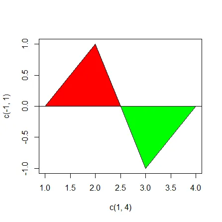
如果你想要两种不同的颜色,你需要两个不同的多边形。你可以多次调用多边形函数,或者在你的x和y向量中添加NA值来指示一个新的多边形。R不会为你自动计算交集。你必须自己完成。下面是如何用不同的颜色绘制它的方法。
x <- c(1,2,2.5,NA,2.5,3,4)
y <- c(0,1,0,NA,0,-1,0)
g <- cumsum(is.na(x))
gc <- ifelse(tapply(y, g,
function(x) x[which.max(abs(x))])>0,
"red","green")
plot(c(1, 4),c(-1,1), type = "n")
polygon(x, y, col = gc)
abline(h=0)
在更一般的情况下,将多边形分成不同的区域可能并不容易。在GIS软件包中,似乎有些支持此类型操作,因为这种操作更为常见。然而,我已经考虑了一个相对简单的多边形情况。
首先,我定义了一个闭包来定义切割线。该函数将取得直线的斜率和截距,并返回我们需要切割多边形所需的函数。
getSplitLine <- function(m=1, b=0) {
    force(m); force(b)
    classify <- function(x,y) {
        y >= m*x + b
    }
    intercepts <- function(x,y, class=classify(x,y)) {
        w <- which(diff(class)!=0)
        m2 <- (y[w+1]-y[w])/(x[w+1]-x[w])
        b2 <- y[w] - m2*x[w]

        ix <- (b2-b)/(m-m2)
        iy <- ix*m + b
        data.frame(x=ix,y=iy,idx=w+.5, dir=((rank(ix, ties="first")+1) %/% 2) %% 2 +1)
    }
    plot <- function(...) {
    abline(b,m,...)
    }
    list(
        intercepts=intercepts,
        classify=classify,
        plot=plot
    )
}
现在,我们将定义一个函数,使用刚刚定义的分割器来实际分割多边形。
splitPolygon <- function(x, y, splitter) {
    addnullrow <- function(x) if (!all(is.na(x[nrow(x),]))) rbind(x, NA) else x
    rollup <- function(x,i=1) rbind(x[(i+1):nrow(x),], x[1:i,])
    idx <- cumsum(is.na(x) | is.na(y))
    polys <- split(data.frame(x=x,y=y)[!is.na(x),], idx[!is.na(x)])
    r <- lapply(polys, function(P) {
        x <- P$x; y<-P$y
        side <- splitter$classify(x, y)
        if(side[1] != side[length(side)]) {
            ints <- splitter$intercepts(c(x,x[1]), c(y, y[1]), c(side, side[1]))
        } else {
            ints <- splitter$intercepts(x, y, side)
        }
        sideps <- lapply(unique(side), function(ss) {
            pts <- data.frame(x=x[side==ss], y=y[side==ss],
                idx=seq_along(x)[side==ss], dir=0)
            mm <- rbind(pts, ints)
            mm <- mm[order(mm$idx), ]
            br <- cumsum(mm$dir!=0 & c(0,head(mm$dir,-1))!=0 &
                c(0,diff(mm$idx))>1)
            if (length(unique(br))>1) {
                mm<-rollup(mm, sum(br==br[1]))
            }
            br <- cumsum(c(FALSE,abs(diff(mm$dir*mm$dir))==3))
            do.call(rbind, lapply(split(mm, br), addnullrow))
        })
        pss<-rep(unique(side), sapply(sideps, nrow))
        ps<-do.call(rbind, lapply(sideps, addnullrow))[,c("x","y")]
        attr(ps, "side")<-pss
        ps
   })
   pss<-unname(unlist(lapply(r, attr, "side")))
   src <- rep(seq_along(r), sapply(r, nrow))
   r <- do.call(rbind, r)
   attr(r, "source")<-src
   attr(r, "side")<-pss
   r
}
输入只是像您将传递给多边形一样的x和y的值,以及切割器。它将返回一个数据框,其中包含可与polygon一起使用的x和y值。
例如:
x <- c(1,2,2.5,NA,2.5,3,4)
y <- c(1,-2,2,NA,-1,2,-2)

sl<-getSplitLine(0,0)

plot(range(x, na.rm=T),range(y, na.rm=T), type = "n")
p <- splitPolygon(x,y,sl)
g <- cumsum(c(F, is.na(head(p$y,-1))))
gc <- ifelse(attr(p,"side")[is.na(p$y)],
    "red","green")
polygon(p, col=gc)
sl$plot(lty=2, col="grey")
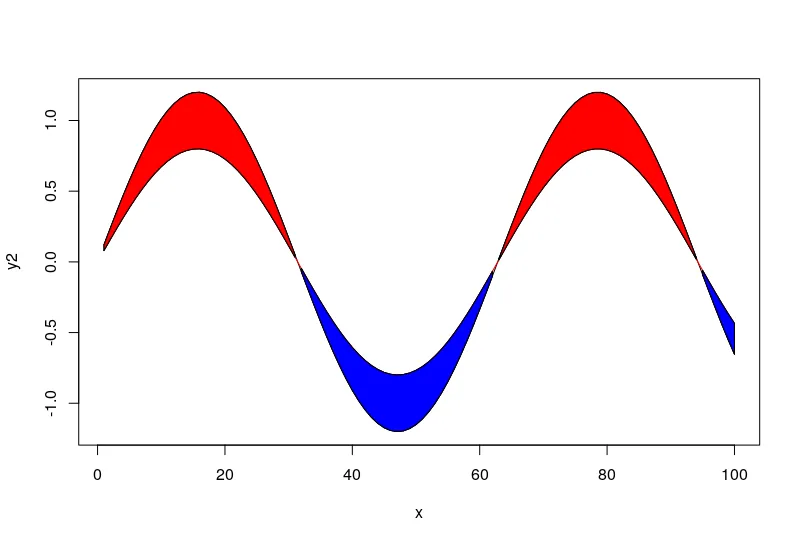
这对于有斜线的简单凸多边形也适用。这里是另一个例子。
x <- c(1,2,3,4,5,4,3,2)
y <- c(-2,2,1,2,-2,.5,-.5,.5)

sl<-getSplitLine(.5,-1.25)

plot(range(x, na.rm=T),range(y, na.rm=T), type = "n")
p <- splitPolygon(x,y,sl)
g <- cumsum(c(F, is.na(head(p$y,-1))))
gc <- ifelse(attr(p,"side")[is.na(p$y)],
    "red","green")
polygon(p, col=gc)
sl$plot(lty=2, col="grey")

目前,当多边形的顶点恰好落在切割线上时,情况可能会有点混乱。我将来可能会尝试修正这个问题。
y中有0,多边形的一侧已经在分割线上了。那么没有0的数据怎么办,比如y <- c(1,-2,2,NA,-1,2,-2)?我不知道需要做出什么样的调整。 - mrub