在我之前的回答中,我思考了一下,想出了一种更简单的方法来生成多面板(如果适用)风扇图,并叠加在 levelplot 上,如维基百科风扇图页面所示。此方法适用于具有两个独立变量和零个或多个调节变量将数据分成面板的 data.frame。
首先,我们定义一个新的面板函数,panel.fanplot。
panel.fanplot <- function(x, y, z, zmin, zmax, subscripts, groups,
nmax=max(tapply(z, list(x, y, groups),
function(x) sum(!is.na(x))), na.rm=T),
...) {
if(missing(zmin)) zmin <- min(z, na.rm=TRUE)
if(missing(zmin)) zmax <- max(z, na.rm=TRUE)
get.coords <- function(a, d, x0, y0) {
a <- ifelse(a <= 90, 90 - a, 450 - a)
data.frame(x = x0 + d * cos(a / 180 * pi),
y = y0 + d * sin(a / 180 * pi))
}
z.scld <- (z - zmin)/(zmax - zmin) * 360
fan <- aggregate(list(z=z.scld[subscripts]),
list(x=x[subscripts], y=y[subscripts]),
function(x)
c(n=sum(!is.na(x)),
quantile(x, c(0.25, 0.5, 0.75), na.rm=TRUE) - 90))
panel.levelplot(fan$x, fan$y,
(fan$z[, '50%'] + 90) / 360 * (zmax - zmin) + zmin,
subscripts=seq_along(fan$x), ...)
lapply(which(!is.na(fan$z[, '50%'])), function(i) {
with(fan[i, ], {
poly <- rbind(c(x, y),
get.coords(seq(z[, '25%'], z[, '75%'], length.out=200),
0.3, x, y))
lpolygon(poly$x, poly$y, col='gray10', border='gray10', lwd=3)
llines(get.coords(c(z[, '50%'], 180 + z[, '50%']), 0.3, x, y),
col='black', lwd=3, lend=1)
llines(get.coords(z[, '50%'], c(0.3, (1 - z[, 'n']/nmax) * 0.3), x, y),
col='white', lwd=3)
})
})
}
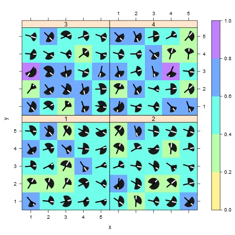
现在我们创建一些虚拟数据并调用
levelplot:
d <- data.frame(z=runif(1000),
x=sample(5, 1000, replace=TRUE),
y=sample(5, 1000, replace=TRUE),
grp=sample(4, 1000, replace=TRUE))
colramp <- colorRampPalette(c('#fff495', '#bbffaa', '#70ffeb', '#72aaff',
'#bf80ff'))
levelplot(z ~ x*y|as.factor(grp), d, groups=grp, asp=1, col.regions=colramp,
panel=panel.fanplot, zmin=min(d$z, na.rm=TRUE),
zmax=max(d$z, na.rm=TRUE), at=seq(0, 1, 0.2))
重要的是通过参数
group将筛选变量(将图形分成面板)传递给
levelplot,如上所示使用变量
grp,以便计算样本大小(由白线长度表示)。
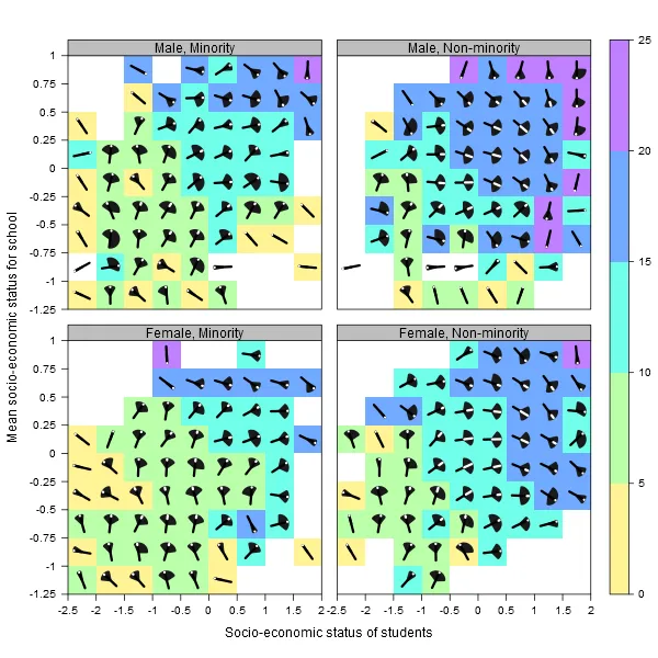
以下是如何模仿维基百科的情况:
library(nlme)
data(MathAchieve)
MathAchieve$SESfac <- as.numeric(cut(MathAchieve$SES, seq(-2.5, 2, 0.5)))
MathAchieve$MEANSESfac <- as.numeric(cut(MathAchieve$MEANSES,
                                         seq(-1.25, 1, 0.25)))
levels(MathAchieve$Minority) <- c('Non-minority', 'Minority')
MathAchieve$group <-
as.factor(paste0(MathAchieve$Sex, ', ', MathAchieve$Minority))
colramp <- colorRampPalette(c('#fff495', '#bbffaa', '#70ffeb', '#72aaff',
                              '#bf80ff'))
levelplot(MathAch ~ SESfac*MEANSESfac|group, MathAchieve,
groups=group, asp=1, col.regions=colramp,
panel=panel.fanplot, zmin=0, zmax=28, at=seq(0, 25, 5),
scales=list(alternating=1,
tck=c(1, 0),
x=list(at=seq(1, 11) - 0.5,
labels=seq(-2.5, 2, 0.5)),
y=list(at=seq(1, 11) - 0.5,
labels=seq(-1.25, 1, 0.25))),
between=list(x=1, y=1), strip=strip.custom(bg='gray'),
xlab='Socio-economic status of students',
ylab='Mean socio-economic status for school')
plotrix包具有大量专业的图表功能。 - IRTFM