我写了下面这个函数,可以制作自定义的堆叠图:
现在,我想将其与以下数据一起使用:
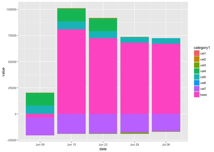
那么我将做出以下这个图表:
stacked_plot <- function(data, what, by = NULL, date_col = date, date_unit = NULL, type = 'area'){

  by <- enquo(by)
  what <- ensym(what)
  date_col <- ensym(date_col)
  date_unit <- enquo(date_unit)

  if (!rlang::as_string(date_col) %in% names(data)){
    return(cat('Nie odnaleziono kolumny "', as_string(date_col), '".', sep = ''))
  }

  if (!rlang::quo_is_null(date_unit)){
    data <- data %>%
      mutate(!!date_col := floor_date(!!date_col, unit = !!date_unit, week_start = 1))
  }

  if (!rlang::quo_is_null(by)) {
    data <- data %>%
      filter(!is.na(!!by)) %>%
      group_by(!!date_col, !!by) %>%
      summarise(!!what := sum(!!what, na.rm = TRUE)) %>%
      ungroup() %>%
      complete(!!date_col, !!by, fill = rlang::list2(!!what := 0))
  } else {
    data <- data %>%
      group_by(!!date_col) %>%
      summarise(!!what := sum(!!what, na.rm = TRUE)) %>%
      complete(!!date_col, fill = rlang::list2(!!what := 0))
  }

  if (type == 'area'){
    p <- data %>%
      ggplot(aes(!!date_col, !!what, fill = !!by)) +
      geom_area(position = 'stack')
  } else if (type == 'col'){
    p <- data %>%
      ggplot(aes(!!date_col, !!what, fill = !!by)) +
      geom_col(position = 'stack')
  }

  p <- p +
    scale_x_date(breaks = '1 month', date_labels = '%Y-%m', expand = c(.01, .01)) +
    theme_minimal() +
    theme(axis.text.x = element_text(angle = 90, vjust = .4)) +
    labs(fill = '')

  return(p)
}
现在,我想将其与以下数据一起使用:
data <- structure(list(category1 = structure(c(7L, 7L, 7L, 7L, 7L, 7L,
7L, 7L, 7L, 7L, 7L, 7L, 7L, 7L, 7L, 7L, 7L, 2L, 1L, 8L, 1L, 1L,
1L, 1L, 6L, 6L, 5L, 5L, 1L, 1L, 8L, 3L, 1L, 1L, 8L, 1L, 1L, 1L,
1L, 1L, 1L, 4L, 7L, 7L, 7L, 7L, 7L, 7L, 7L, 7L, 7L, 7L, 7L, 7L,
7L, 7L, 7L, 7L, 7L, 7L, 2L, 1L, 8L, 1L, 1L, 1L, 1L, 6L, 6L, 5L,
5L, 1L, 1L, 8L, 3L, 1L, 1L, 8L, 1L, 1L, 1L, 1L, 1L, 1L, 4L, 7L,
7L, 7L, 7L, 7L, 7L, 7L, 7L, 7L, 7L, 7L, 7L, 7L, 7L, 7L, 7L, 7L,
7L, 2L, 1L, 8L, 1L, 1L, 1L, 1L, 6L, 6L, 5L, 5L, 1L, 1L, 8L, 3L,
1L, 1L, 8L, 1L, 1L, 1L, 1L, 1L, 1L, 4L, 7L, 7L, 7L, 7L, 7L, 7L,
7L, 7L, 7L, 7L, 7L, 7L, 7L, 7L, 7L, 7L, 7L, 7L, 2L, 1L, 8L, 1L,
1L, 1L, 1L, 6L, 6L, 5L, 5L, 1L, 1L, 8L, 3L, 1L, 1L, 8L, 1L, 1L,
1L, 1L, 1L, 1L, 4L, 7L, 7L, 7L, 7L, 7L, 7L, 7L, 7L, 7L, 7L, 7L,
7L, 7L, 7L, 7L, 7L, 7L, 7L, 2L, 1L, 8L, 1L, 1L, 1L, 1L, 6L, 6L,
5L, 5L, 1L), .Label = c("base", "cat1", "cat2", "cat3", "cat4",
"cat5", "cat6", "cat7"), class = "factor"), date = structure(c(14403,
14403, 14403, 14403, 14403, 14403, 14403, 14403, 14403, 14403,
14403, 14403, 14403, 14403, 14403, 14403, 14403, 14403, 14403,
14403, 14403, 14403, 14403, 14403, 14403, 14403, 14403, 14403,
14403, 14403, 14403, 14403, 14403, 14410, 14410, 14410, 14410,
14410, 14410, 14410, 14410, 14410, 14410, 14410, 14410, 14410,
14410, 14410, 14410, 14410, 14410, 14410, 14410, 14410, 14410,
14410, 14410, 14410, 14410, 14410, 14410, 14410, 14410, 14410,
14410, 14410, 14410, 14410, 14410, 14410, 14410, 14410, 14410,
14410, 14410, 14410, 14417, 14417, 14417, 14417, 14417, 14417,
14417, 14417, 14417, 14417, 14417, 14417, 14417, 14417, 14417,
14417, 14417, 14417, 14417, 14417, 14417, 14417, 14417, 14417,
14417, 14417, 14417, 14417, 14417, 14417, 14417, 14417, 14417,
14417, 14417, 14417, 14417, 14417, 14417, 14417, 14417, 14417,
14417, 14424, 14424, 14424, 14424, 14424, 14424, 14424, 14424,
14424, 14424, 14424, 14424, 14424, 14424, 14424, 14424, 14424,
14424, 14424, 14424, 14424, 14424, 14424, 14424, 14424, 14424,
14424, 14424, 14424, 14424, 14424, 14424, 14424, 14424, 14424,
14424, 14424, 14424, 14424, 14424, 14424, 14424, 14424, 14431,
14431, 14431, 14431, 14431, 14431, 14431, 14431, 14431, 14431,
14431, 14431, 14431, 14431, 14431, 14431, 14431, 14431, 14431,
14431, 14431, 14431, 14431, 14431, 14431, 14431, 14431, 14431,
14431, 14431, 14431, 14431, 14431, 14431, 14431, 14431, 14431,
14431, 14431), class = "Date"), value = c(0.0296166578938365,
7.02892806393191e-05, 0, 0, 0, 0, 0, 0, 0, 0, 0, 0, 0, 0, 0,
0, 0, -23.1966033032737, 0, -17195.0853457778, 0, 0, 0, 0, 0,
7861.28404641463, 12189.6349251651, 0, 0, -3741.93702617252,
0, 176.303827249194, 391.710849761278, 131970.980379196, -1587.22123177257,
297.978554303167, -51860.1739251141, 0, 0, 0, 0, -391.332709445819,
0.000172964963558834, 0.0098722192979455, 2.34186560613466e-05,
0, 0, 0, 0, 0, 0, 0, 0, 0, 0, 0, 0, 0, 0, 0, -7.73219962306076,
0, -17218.0930016352, 0, 0, 0, 0, 0, 7781.23968988082, 12189.6349251651,
0, 0, 0, 0, 449.478850296707, 293.783137320959, 131970.980379196,
-1404.7589064091, 250.836431075847, -56540.9156671359, 0, 0,
0, 0, -558.95740304599, 5.77335368827169e-05, 0.00329073976598183,
7.79511453535577e-06, 0, 0, 0, 0, 0, 0, 0, 0, 0, 0, 0, 0, 0,
0, 0, -2.57739987435359, 0, -17241.1006574926, 0, 0, 0, 0, 0,
6598.97373566299, 12189.6349251651, 0, -3324.25546024928, 0,
0, 549.603379062553, 195.855424880639, 131970.980379196, -529.148187957385,
219.828510450391, -64437.2982346174, 0, 0, 0, 0, -1447.22409849783,
1.92288024882845e-05, 0.00109691325532728, 2.60503400284112e-06,
0, 0, 0, 0, 0, 0, 0, 0, 0, 0, 0, 0, 0, 0, 0, -0.859131813420729,
0, -17264.10831335, 0, 0, 0, 0, 0, 5437.37054226604, 0, 0, 0,
0, 0, 293.381058210822, 293.783137320959, 131970.980379196, 526.728756878514,
207.979955414647, -65107.9475533677, 0, 0, 0, 0, -336.514645781955,
6.40960082942816e-06, 0.000366094798965479, 8.69455082789682e-07,
0, 0, 0, 0, 0, 0, 0, 0, 0, 0, 0, 0, 0, 0, 0, -127.057071107617,
0, -17287.1159692073, 0, 0, 0, 0, 0, 5343.46624155083, 0, 0,
0)), class = "data.frame", row.names = c(NA, -201L))
那么我将做出以下这个图表:
data %>% stacked_plot(value, category1, date, type = 'col')
我的问题在于,我无法确定我的因子变量(category1)的堆叠顺序。我想要做的是在函数内重新排序因子水平,使得base类别始终以0开头,并将其余水平层叠在其上或下方。好吧,它不一定总是命名为base,但我认为我们可以在函数中添加一个参数,并向其提供base变量的名称。当然,输入数据文件可以有不同数量的类别。