期望最大化算法(Expectation Maximization,简称EM)是一种用于分类数据的概率方法。如果它不属于分类器,请纠正我。
这个EM技术的直观解释是什么?这里的“期望”是什么,什么被“最大化”了?
期望最大化算法(Expectation Maximization,简称EM)是一种用于分类数据的概率方法。如果它不属于分类器,请纠正我。
这个EM技术的直观解释是什么?这里的“期望”是什么,什么被“最大化”了?
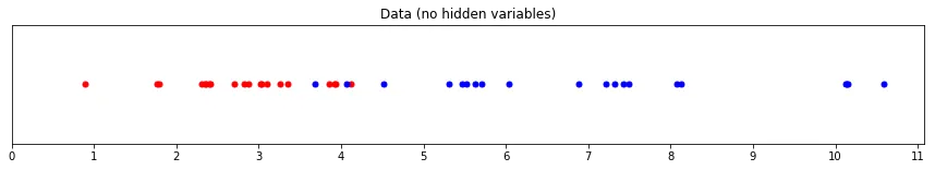
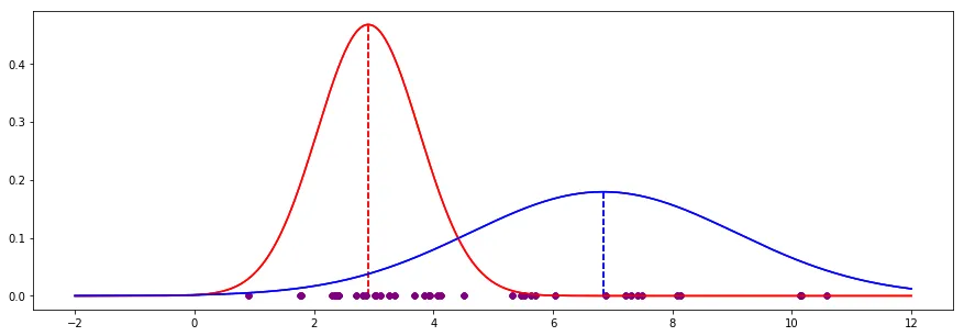
假设我们有两个不同组别的数据,红色和蓝色:
import numpy as np
from scipy import stats

np.random.seed(110) # for reproducible results

# set parameters
red_mean = 3
red_std = 0.8

blue_mean = 7
blue_std = 2

# draw 20 samples from normal distributions with red/blue parameters
red = np.random.normal(red_mean, red_std, size=20)
blue = np.random.normal(blue_mean, blue_std, size=20)

both_colours = np.sort(np.concatenate((red, blue))) # for later use...
这里再次展示红色和蓝色组的图像(为了避免您需要向上滚动):
>>> np.mean(red)
2.802
>>> np.std(red)
0.871
>>> np.mean(blue)
6.932
>>> np.std(blue)
2.195
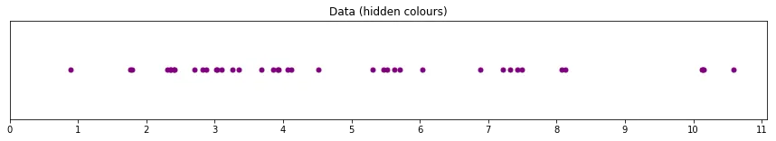
如果我们看不到点的颜色怎么办?也就是说,每个点都被染成了紫色,而不是红色或蓝色。
为了尝试恢复红色和蓝色组的平均值和标准差参数,我们可以使用期望最大化算法。
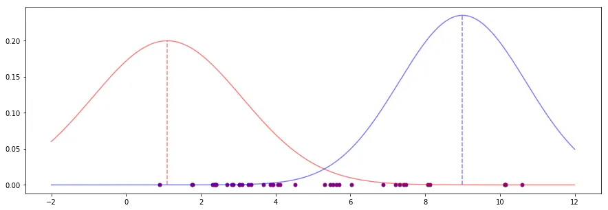
我们的第一步(上面的步骤1)是猜测每个组的平均值和标准差参数值。我们不必进行明智的猜测;我们可以选择任何数字:
# estimates for the mean
red_mean_guess = 1.1
blue_mean_guess = 9

# estimates for the standard deviation
red_std_guess = 2
blue_std_guess = 1.7
likelihood_of_red = stats.norm(red_mean_guess, red_std_guess).pdf(both_colours)
likelihood_of_blue = stats.norm(blue_mean_guess, blue_std_guess).pdf(both_colours)
likelihood_total = likelihood_of_red + likelihood_of_blue

red_weight = likelihood_of_red / likelihood_total
blue_weight = likelihood_of_blue / likelihood_total
def estimate_mean(data, weight):
    """
    For each data point, multiply the point by the probability it
    was drawn from the colour's distribution (its "weight").

    Divide by the total weight: essentially, we're finding where
    the weight is centred among our data points.
    """
    return np.sum(data * weight) / np.sum(weight)

def estimate_std(data, weight, mean):
    """
    For each data point, multiply the point's squared difference
    from a mean value by the probability it was drawn from
    that distribution (its "weight").

    Divide by the total weight: essentially, we're finding where
    the weight is centred among the values for the difference of
    each data point from the mean.

    This is the estimate of the variance, take the positive square
    root to find the standard deviation.
    """
    variance = np.sum(weight * (data - mean)**2) / np.sum(weight)
    return np.sqrt(variance)

# new estimates for standard deviation
blue_std_guess = estimate_std(both_colours, blue_weight, blue_mean_guess)
red_std_guess = estimate_std(both_colours, red_weight, red_mean_guess)

# new estimates for mean
red_mean_guess = estimate_mean(both_colours, red_weight)
blue_mean_guess = estimate_mean(both_colours, blue_weight)
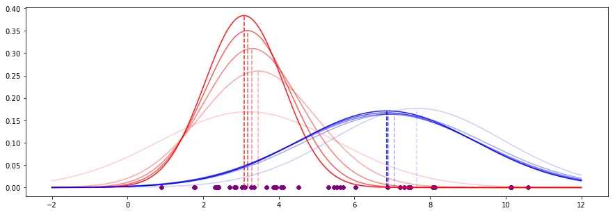
          | EM guess | Actual |  Delta
----------+----------+--------+-------
Red mean  |    2.910 |  2.802 |  0.108
Red std   |    0.854 |  0.871 | -0.017
Blue mean |    6.838 |  6.932 | -0.094
Blue std  |    2.227 |  2.195 |  0.032
EM是一种算法,用于在模型中存在未观测变量(即潜在变量)时,最大化似然函数。
你可能会问,如果我们只是试图最大化一个函数,为什么不使用现有的最大化函数的工具呢?嗯,如果您尝试通过对导数取零来最大化它,在许多情况下,一阶条件没有解。这里存在一个鸡生蛋的问题,要解决模型参数,需要知道未观测数据的分布,但未观测数据的分布是模型参数的函数。
E-M试图通过迭代地猜测未观测数据的分布,然后通过最大化某个低于实际似然函数的下限的东西来估计模型参数,并重复此过程直到收敛:
EM算法
从您的模型参数值开始猜想
E步骤:对于每个具有缺失值的数据点,请使用模型方程解出给定您当前模型参数和给定观测数据的情况下缺失数据的分布(请注意,您正在为每个缺失值解决一个分布,而不是期望值)。由于我们已经有了每个缺失值的分布,因此我们可以根据未观测变量计算似然函数的期望值。如果我们对模型参数的猜测是正确的,那么这个期望似然将是我们观察数据的实际似然;如果参数不正确,它只是一个下限。
M步骤:现在,我们已经得到了没有未观测变量的期望似然函数,请像在完全观测的情况下一样最大化该函数,以获得模型参数的新估计。
重复直到收敛。
这是一个简单的食谱,用于理解期望最大化算法:
1- 阅读Do和Batzoglou的EM教程论文。
2- 如果你脑海中有问号,可以查看这个数学堆栈交流页面上的解释。
3- 查看我在Python中编写的代码,它解释了第1项的EM教程论文中的示例:
警告: 代码可能有些混乱/不太优化,因为我不是Python开发人员。但它能够完成任务。
import numpy as np
import math

#### E-M Coin Toss Example as given in the EM tutorial paper by Do and Batzoglou* ####

def get_mn_log_likelihood(obs,probs):
    """ Return the (log)likelihood of obs, given the probs"""
    # Multinomial Distribution Log PMF
    # ln (pdf)      =             multinomial coeff            *   product of probabilities
    # ln[f(x|n, p)] = [ln(n!) - (ln(x1!)+ln(x2!)+...+ln(xk!))] + [x1*ln(p1)+x2*ln(p2)+...+xk*ln(pk)]

    multinomial_coeff_denom= 0
    prod_probs = 0
    for x in range(0,len(obs)): # loop through state counts in each observation
        multinomial_coeff_denom = multinomial_coeff_denom + math.log(math.factorial(obs[x]))
        prod_probs = prod_probs + obs[x]*math.log(probs[x])

    multinomial_coeff = math.log(math.factorial(sum(obs))) -  multinomial_coeff_denom
    likelihood = multinomial_coeff + prod_probs
    return likelihood

# 1st:  Coin B, {HTTTHHTHTH}, 5H,5T
# 2nd:  Coin A, {HHHHTHHHHH}, 9H,1T
# 3rd:  Coin A, {HTHHHHHTHH}, 8H,2T
# 4th:  Coin B, {HTHTTTHHTT}, 4H,6T
# 5th:  Coin A, {THHHTHHHTH}, 7H,3T
# so, from MLE: pA(heads) = 0.80 and pB(heads)=0.45

# represent the experiments
head_counts = np.array([5,9,8,4,7])
tail_counts = 10-head_counts
experiments = zip(head_counts,tail_counts)

# initialise the pA(heads) and pB(heads)
pA_heads = np.zeros(100); pA_heads[0] = 0.60
pB_heads = np.zeros(100); pB_heads[0] = 0.50

# E-M begins!
delta = 0.001
j = 0 # iteration counter
improvement = float('inf')
while (improvement>delta):
    expectation_A = np.zeros((5,2), dtype=float)
    expectation_B = np.zeros((5,2), dtype=float)
    for i in range(0,len(experiments)):
        e = experiments[i] # i'th experiment
        ll_A = get_mn_log_likelihood(e,np.array([pA_heads[j],1-pA_heads[j]])) # loglikelihood of e given coin A
        ll_B = get_mn_log_likelihood(e,np.array([pB_heads[j],1-pB_heads[j]])) # loglikelihood of e given coin B

        weightA = math.exp(ll_A) / ( math.exp(ll_A) + math.exp(ll_B) ) # corresponding weight of A proportional to likelihood of A
        weightB = math.exp(ll_B) / ( math.exp(ll_A) + math.exp(ll_B) ) # corresponding weight of B proportional to likelihood of B

        expectation_A[i] = np.dot(weightA, e)
        expectation_B[i] = np.dot(weightB, e)

    pA_heads[j+1] = sum(expectation_A)[0] / sum(sum(expectation_A));
    pB_heads[j+1] = sum(expectation_B)[0] / sum(sum(expectation_B));

    improvement = max( abs(np.array([pA_heads[j+1],pB_heads[j+1]]) - np.array([pA_heads[j],pB_heads[j]]) ))
    j = j+1
从技术上讲,“EM”这个术语有些不够具体,但我假设你是指高斯混合模型聚类分析技术,它是一种通用EM原理的实例。
实际上,EM聚类分析不是分类器。我知道有些人认为聚类是“无监督分类”,但实际上聚类分析是完全不同的东西。
分类和聚类分析之间的关键区别, 以及分类人员总是误解聚类分析的大误解是:在聚类分析中,没有“正确的解决方案”。这是一种知识"发现"方法,实际上是为了找到一些新的东西!这使得评估变得非常棘手。通常使用已知分类作为参考进行评估,但这并不总是适当的:您拥有的分类可能与数据中的情况有所不同。
让我举个例子:您有一个大的客户数据集,包括性别数据。将此数据集分成“男性”和“女性”的方法在与现有类别进行比较时是最优的。从“预测”的思考方式来看,这很好,因为对于新用户,您现在可以预测他们的性别。从“知识发现”的思考方式来看,这实际上是不好的,因为您希望在数据中发现一些新结构。例如,将数据分成老年人和儿童将得到一个最差的聚类结果(如果没有给出年龄),但这将是一个出色的聚类结果。
现在回到EM。基本上,它假设您的数据由多个多元正态分布组成(请注意,这是一个非常强的假设,特别是当您固定聚类数时!)。然后,它通过交替改进模型和对象分配到模型来寻找局部最优模型。
在分类背景下获得最佳结果,请选择聚类数量比类别数量大,甚至仅对单个类别应用聚类分析(以查找类别内是否存在某些结构!)。
假设你想训练一个分类器来区分“汽车”、“自行车”和“卡车”。 假设数据不仅仅由三个正态分布组成并没有太大用处。 但是,您可以假设 存在多种类型的汽车(以及卡车和自行车)。 因此,不是为这三个类别培训分类器,而是将汽车、卡车和自行车分别聚类成10个簇(或者可能是10辆汽车,3辆卡车和3辆自行车等),然后训练一个分类器来区分这30个类别,然后将识别结果合并回原始类别。 您也可能发现有一个特别难以分类的簇,例如三轮车。 它们有点像汽车,有点像自行车。 或者送货卡车,更像是超大型汽车而不是卡车。被接受的答案参考了Chuong EM Paper,该论文很好地解释了EM。还有一个YouTube视频更详细地解释了这篇论文。
总之,这里是情景:
1st:  {H,T,T,T,H,H,T,H,T,H} 5 Heads, 5 Tails; Did coin A or B generate me?
2nd:  {H,H,H,H,T,H,H,H,H,H} 9 Heads, 1 Tails
3rd:  {H,T,H,H,H,H,H,T,H,H} 8 Heads, 2 Tails
4th:  {H,T,H,T,T,T,H,H,T,T} 4 Heads, 6 Tails
5th:  {T,H,H,H,T,H,H,H,T,H} 7 Heads, 3 Tails

Two possible coins, A & B are used to generate these distributions.
A & B have an unknown parameter: their bias towards heads.

We don't know the biases, but we can simply start with a guess: A=60% heads, B=50% heads.
注意:当这种算法收敛到(全局)最优解时,它已经找到了一个在x和y两个参数领域中都是最好的配置。然而,该算法可能只能找到一个局部最优解而不是全局最优解。
我会说这是算法概述的直观描述。
对于统计论证和应用,其他答案提供了很好的解释(还可以检查本答案中的参考文献)。
使用Zhubarb答案中引用的Do和Batzoglou的文章,我在Java中实现了EM算法来解决该问题。他回答中的评论显示,如果参数thetaA和thetaB相同,则该算法会陷入局部最优解,我的实现也会出现这种情况。
下面是我的代码的标准输出,显示参数的收敛情况。
thetaA = 0.71301, thetaB = 0.58134
thetaA = 0.74529, thetaB = 0.56926
thetaA = 0.76810, thetaB = 0.54954
thetaA = 0.78316, thetaB = 0.53462
thetaA = 0.79106, thetaB = 0.52628
thetaA = 0.79453, thetaB = 0.52239
thetaA = 0.79593, thetaB = 0.52073
thetaA = 0.79647, thetaB = 0.52005
thetaA = 0.79667, thetaB = 0.51977
thetaA = 0.79674, thetaB = 0.51966
thetaA = 0.79677, thetaB = 0.51961
thetaA = 0.79678, thetaB = 0.51960
thetaA = 0.79679, thetaB = 0.51959
Final result:
thetaA = 0.79678, thetaB = 0.51960
private Parameters _parameters;

public Parameters run()
{
    while (true)
    {
        expectation();

        Parameters estimatedParameters = maximization();

        if (_parameters.converged(estimatedParameters)) {
            break;
        }

        _parameters = estimatedParameters;
    }

    return _parameters;
}
import java.util.*;

/*****************************************************************************
This class encapsulates the parameters of the problem. For this problem posed
in the article by (Do and Batzoglou, 2008), the parameters are thetaA and
thetaB, the probability of a coin coming up heads for the two coins A and B,
respectively.
*****************************************************************************/
class Parameters
{
    double _thetaA = 0.0; // Probability of heads for coin A.
    double _thetaB = 0.0; // Probability of heads for coin B.

    double _delta = 0.00001;

    public Parameters(double thetaA, double thetaB)
    {
        _thetaA = thetaA;
        _thetaB = thetaB;
    }

    /*************************************************************************
    Returns true if this parameter is close enough to another parameter
    (typically the estimated parameter coming from the maximization step).
    *************************************************************************/
    public boolean converged(Parameters other)
    {
        if (Math.abs(_thetaA - other._thetaA) < _delta &&
            Math.abs(_thetaB - other._thetaB) < _delta)
        {
            return true;
        }

        return false;
    }

    public double getThetaA()
    {
        return _thetaA;
    }

    public double getThetaB()
    {
        return _thetaB;
    }

    public String toString()
    {
        return String.format("thetaA = %.5f, thetaB = %.5f", _thetaA, _thetaB);
    }

}


/*****************************************************************************
This class encapsulates an observation, that is the number of heads
and tails in a trial. The observation can be either (1) one of the
experimental observations, or (2) an estimated observation resulting from
the expectation step.
*****************************************************************************/
class Observation
{
    double _numHeads = 0;
    double _numTails = 0;

    public Observation(String s)
    {
        for (int i = 0; i < s.length(); i++)
        {
            char c = s.charAt(i);

            if (c == 'H')
            {
                _numHeads++;
            }
            else if (c == 'T')
            {
                _numTails++;
            }
            else
            {
                throw new RuntimeException("Unknown character: " + c);
            }
        }
    }

    public Observation(double numHeads, double numTails)
    {
        _numHeads = numHeads;
        _numTails = numTails;
    }

    public double getNumHeads()
    {
        return _numHeads;
    }

    public double getNumTails()
    {
        return _numTails;
    }

    public String toString()
    {
        return String.format("heads: %.1f, tails: %.1f", _numHeads, _numTails);
    }

}

/*****************************************************************************
This class runs expectation-maximization for the problem posed by the article
from (Do and Batzoglou, 2008).
*****************************************************************************/
public class EM
{
    // Current estimated parameters.
    private Parameters _parameters;

    // Observations from the trials. These observations are set once.
    private final List<Observation> _observations;

    // Estimated observations per coin. These observations are the output
    // of the expectation step.
    private List<Observation> _expectedObservationsForCoinA;
    private List<Observation> _expectedObservationsForCoinB;

    private static java.io.PrintStream o = System.out;

    /*************************************************************************
    Principal constructor.
    @param observations The observations from the trial.
    @param parameters The initial guessed parameters.
    *************************************************************************/
    public EM(List<Observation> observations, Parameters parameters)
    {
        _observations = observations;
        _parameters = parameters;
    }

    /*************************************************************************
    Run EM until parameters converge.
    *************************************************************************/
    public Parameters run()
    {

        while (true)
        {
            expectation();

            Parameters estimatedParameters = maximization();

            o.printf("%s\n", estimatedParameters);

            if (_parameters.converged(estimatedParameters)) {
                break;
            }

            _parameters = estimatedParameters;
        }

        return _parameters;

    }

    /*************************************************************************
    Given the observations and current estimated parameters, compute new
    estimated completions (distribution over the classes) and observations.
    *************************************************************************/
    private void expectation()
    {

        _expectedObservationsForCoinA = new ArrayList<Observation>();
        _expectedObservationsForCoinB = new ArrayList<Observation>();

        for (Observation observation : _observations)
        {
            int numHeads = (int)observation.getNumHeads();
            int numTails = (int)observation.getNumTails();

            double probabilityOfObservationForCoinA=
                binomialProbability(10, numHeads, _parameters.getThetaA());

            double probabilityOfObservationForCoinB=
                binomialProbability(10, numHeads, _parameters.getThetaB());

            double normalizer = probabilityOfObservationForCoinA +
                                probabilityOfObservationForCoinB;

            // Compute the completions for coin A and B (i.e. the probability
            // distribution of the two classes, summed to 1.0).

            double completionCoinA = probabilityOfObservationForCoinA /
                                     normalizer;
            double completionCoinB = probabilityOfObservationForCoinB /
                                     normalizer;

            // Compute new expected observations for the two coins.

            Observation expectedObservationForCoinA =
                new Observation(numHeads * completionCoinA,
                                numTails * completionCoinA);

            Observation expectedObservationForCoinB =
                new Observation(numHeads * completionCoinB,
                                numTails * completionCoinB);

            _expectedObservationsForCoinA.add(expectedObservationForCoinA);
            _expectedObservationsForCoinB.add(expectedObservationForCoinB);
        }
    }

    /*************************************************************************
    Given new estimated observations, compute new estimated parameters.
    *************************************************************************/
    private Parameters maximization()
    {

        double sumCoinAHeads = 0.0;
        double sumCoinATails = 0.0;
        double sumCoinBHeads = 0.0;
        double sumCoinBTails = 0.0;

        for (Observation observation : _expectedObservationsForCoinA)
        {
            sumCoinAHeads += observation.getNumHeads();
            sumCoinATails += observation.getNumTails();
        }

        for (Observation observation : _expectedObservationsForCoinB)
        {
            sumCoinBHeads += observation.getNumHeads();
            sumCoinBTails += observation.getNumTails();
        }

        return new Parameters(sumCoinAHeads / (sumCoinAHeads + sumCoinATails),
                              sumCoinBHeads / (sumCoinBHeads + sumCoinBTails));

        //o.printf("parameters: %s\n", _parameters);

    }

    /*************************************************************************
    Since the coin-toss experiment posed in this article is a Bernoulli trial,
    use a binomial probability Pr(X=k; n,p) = (n choose k) * p^k * (1-p)^(n-k).
    *************************************************************************/
    private static double binomialProbability(int n, int k, double p)
    {
        double q = 1.0 - p;
        return nChooseK(n, k) * Math.pow(p, k) * Math.pow(q, n-k);
    }

    private static long nChooseK(int n, int k)
    {
        long numerator = 1;

        for (int i = 0; i < k; i++)
        {
            numerator = numerator * n;
            n--;
        }

        long denominator = factorial(k);

        return (long)(numerator / denominator);
    }

    private static long factorial(int n)
    {
        long result = 1;
        for (; n >0; n--)
        {
            result = result * n;
        }

        return result;
    }

    /*************************************************************************
    Entry point into the program.
    *************************************************************************/
    public static void main(String argv[])
    {
        // Create the observations and initial parameter guess
        // from the (Do and Batzoglou, 2008) article.

        List<Observation> observations = new ArrayList<Observation>();
        observations.add(new Observation("HTTTHHTHTH"));
        observations.add(new Observation("HHHHTHHHHH"));
        observations.add(new Observation("HTHHHHHTHH"));
        observations.add(new Observation("HTHTTTHHTT"));
        observations.add(new Observation("THHHTHHHTH"));

        Parameters initialParameters = new Parameters(0.6, 0.5);

        EM em = new EM(observations, initialParameters);

        Parameters finalParameters = em.run();

        o.printf("Final result:\n%s\n", finalParameters);
    }
}
EM用于最大化具有潜在变量Z的模型Q的可能性。
这是一个迭代优化过程。
theta <- initial guess for hidden parameters
while not converged:
    #e-step
    Q(theta'|theta) = E[log L(theta|Z)]
    #m-step
    theta <- argmax_theta' Q(theta'|theta)
e步骤: 给定当前的Z估计,计算期望的对数似然函数
m步骤: 找到最大化这个Q的theta
GMM示例:
e步骤: 根据当前的gmm参数估计,估计每个数据点的标签分配
m步骤: 在新的标签分配下最大化新的theta
K-means也是EM算法,有很多关于K-means的解释动画。