许多用户引用它作为切换到Pytorch的原因,但我仍然没有找到一个正当的理由/解释来牺牲最重要的实际质量--速度,来进行急切执行。
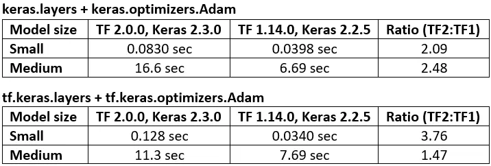
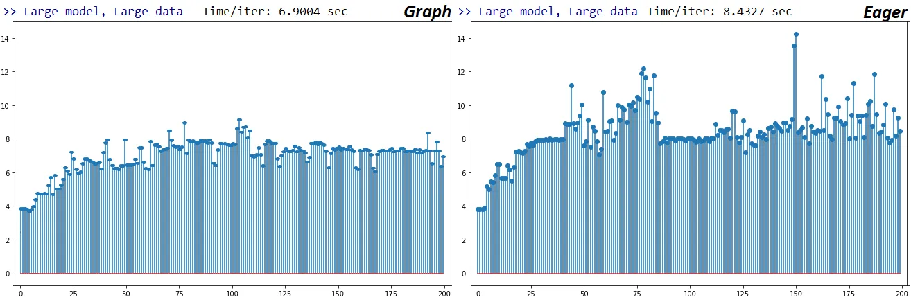
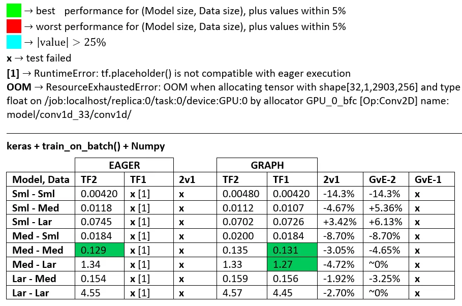
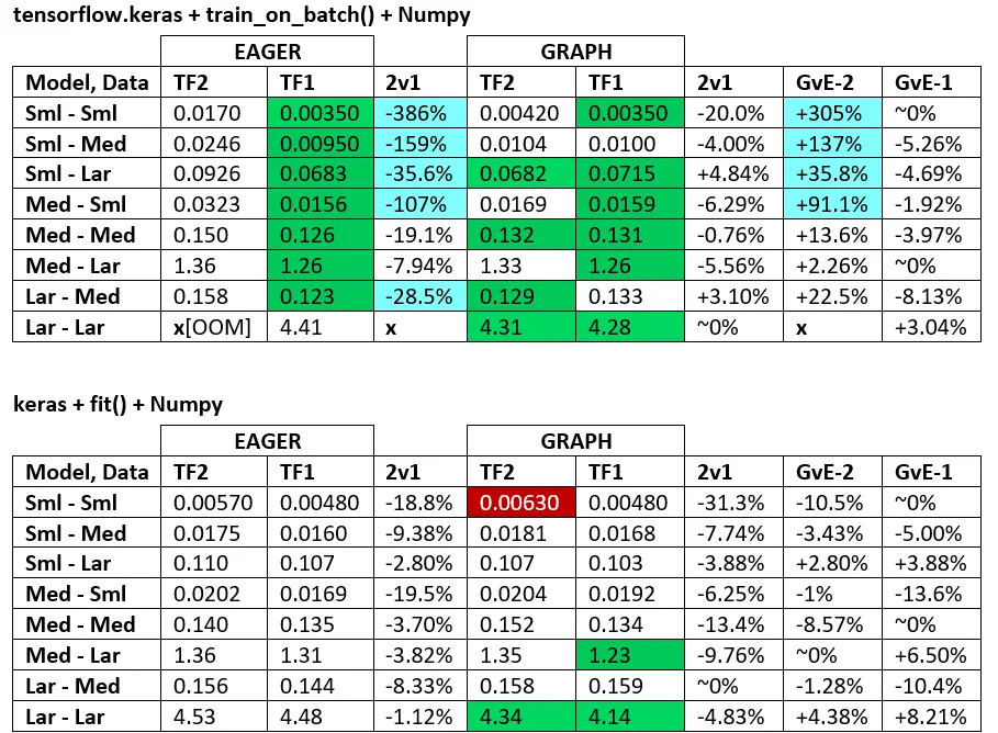
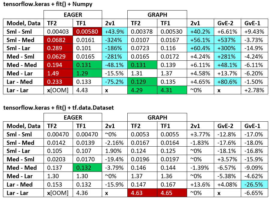
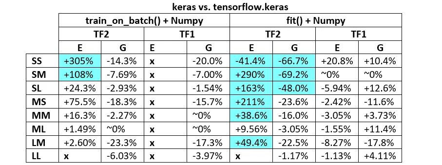
以下是代码基准测试性能,TF1 vs. TF2 - 在TF1上运行速度普遍比TF2快47%至276%。
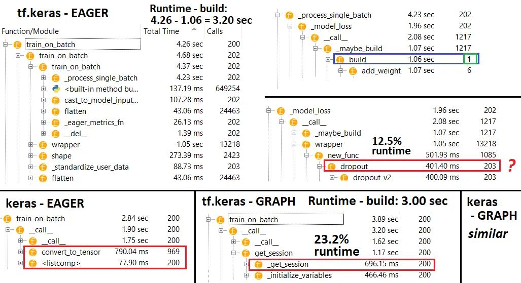
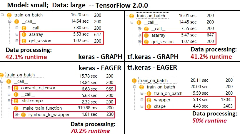
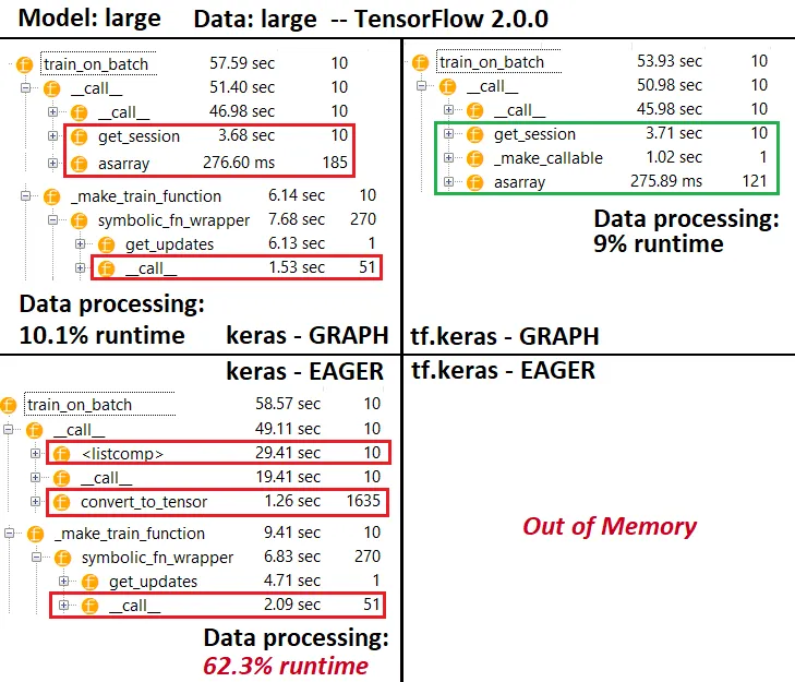
我的问题是:在图形或硬件级别上,是什么导致如此显着的减速?
寻找详细答案- 已经熟悉广泛的概念。有关Git
规格: CUDA 10.0.130, cuDNN 7.4.2, Python 3.7.4, Windows 10, GTX 1070
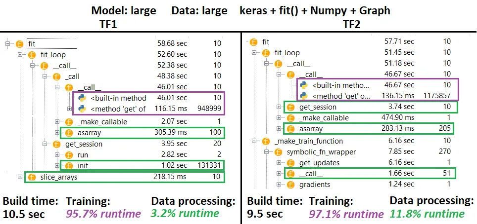
基准测试结果:
更新:根据下面的代码禁用急切执行并不能帮助。然而,行为不一致:有时以图形模式运行会显着提高速度,而其他时候相对于Eager则更慢。
基准测试代码:
# use tensorflow.keras... to benchmark tf.keras; used GPU for all above benchmarks
from keras.layers import Input, Dense, LSTM, Bidirectional, Conv1D
from keras.layers import Flatten, Dropout
from keras.models import Model
from keras.optimizers import Adam
import keras.backend as K
import numpy as np
from time import time

batch_shape = (32, 400, 16)
X, y = make_data(batch_shape)

model_small = make_small_model(batch_shape)
model_small.train_on_batch(X, y)  # skip first iteration which builds graph
timeit(model_small.train_on_batch, 200, X, y)

K.clear_session()  # in my testing, kernel was restarted instead

model_medium = make_medium_model(batch_shape)
model_medium.train_on_batch(X, y)  # skip first iteration which builds graph
timeit(model_medium.train_on_batch, 10, X, y)
使用的函数:
def timeit(func, iterations, *args):
    t0 = time()
    for _ in range(iterations):
        func(*args)
    print("Time/iter: %.4f sec" % ((time() - t0) / iterations))

def make_small_model(batch_shape):
    ipt   = Input(batch_shape=batch_shape)
    x     = Conv1D(128, 400, strides=4, padding='same')(ipt)
    x     = Flatten()(x)
    x     = Dropout(0.5)(x)
    x     = Dense(64, activation='relu')(x)
    out   = Dense(1,  activation='sigmoid')(x)
    model = Model(ipt, out)
    model.compile(Adam(lr=1e-4), 'binary_crossentropy')
    return model

def make_medium_model(batch_shape):
    ipt   = Input(batch_shape=batch_shape)
    x     = Bidirectional(LSTM(512, activation='relu', return_sequences=True))(ipt)
    x     = LSTM(512, activation='relu', return_sequences=True)(x)
    x     = Conv1D(128, 400, strides=4, padding='same')(x)
    x     = Flatten()(x)
    x     = Dense(256, activation='relu')(x)
    x     = Dropout(0.5)(x)
    x     = Dense(128, activation='relu')(x)
    x     = Dense(64,  activation='relu')(x)
    out   = Dense(1,   activation='sigmoid')(x)
    model = Model(ipt, out)
    model.compile(Adam(lr=1e-4), 'binary_crossentropy')
    return model

def make_data(batch_shape):
    return np.random.randn(*batch_shape), np.random.randint(0, 2, (batch_shape[0], 1))