如何找到三次贝塞尔曲线上最接近平面上任意点P的点B(t)?
三次贝塞尔曲线上最接近的点是什么?
53
- Adrian Lopez
4
2这里有一个基本实现的好参考资料:http://www.tinaja.com/glib/bezdist.pdf - drawnonward
2在查看了链接的PDF之后,我认为我正在寻找更加描述性的东西——更像一篇学术论文。就目前而言,我不确定我真正理解所描述的算法到底是做什么的。 - Adrian Lopez
2不涉及距离,但如果您对贝塞尔曲线感兴趣,这是一个有趣的阅读页面:http://www.redpicture.com/bezier/bezier-01.html - drawnonward
2这个http://pomax.github.io/bezierjs/也是一个相关的javascript最近点实现。我最终研究了这个和上一个回答,因为我有一个类似的问题。 - Vlad Nicula
6个回答
28
我编写了一些快速粗糙的代码,可以估算任意次数的贝塞尔曲线。 (注意:这是伪暴力解法,而不是封闭形式的解决方案。)
演示:http://phrogz.net/svg/closest-point-on-bezier.html
/** Find the ~closest point on a Bézier curve to a point you supply.
 * out    : A vector to modify to be the point on the curve
 * curve  : Array of vectors representing control points for a Bézier curve
 * pt     : The point (vector) you want to find out to be near
 * tmps   : Array of temporary vectors (reduces memory allocations)
 * returns: The parameter t representing the location of `out`
 */
function closestPoint(out, curve, pt, tmps) {
    let mindex, scans=25; // More scans -> better chance of being correct
    const vec=vmath['w' in curve[0]?'vec4':'z' in curve[0]?'vec3':'vec2'];
    for (let min=Infinity, i=scans+1;i--;) {
        let d2 = vec.squaredDistance(pt, bézierPoint(out, curve, i/scans, tmps));
        if (d2<min) { min=d2; mindex=i }
    }
    let t0 = Math.max((mindex-1)/scans,0);
    let t1 = Math.min((mindex+1)/scans,1);
    let d2ForT = t => vec.squaredDistance(pt, bézierPoint(out,curve,t,tmps));
    return localMinimum(t0, t1, d2ForT, 1e-4);
}

/** Find a minimum point for a bounded function. May be a local minimum.
 * minX   : the smallest input value
 * maxX   : the largest input value
 * ƒ      : a function that returns a value `y` given an `x`
 * ε      : how close in `x` the bounds must be before returning
 * returns: the `x` value that produces the smallest `y`
 */
function localMinimum(minX, maxX, ƒ, ε) {
    if (ε===undefined) ε=1e-10;
    let m=minX, n=maxX, k;
    while ((n-m)>ε) {
        k = (n+m)/2;
        if (ƒ(k-ε)<ƒ(k+ε)) n=k;
        else               m=k;
    }
    return k;
}

/** Calculate a point along a Bézier segment for a given parameter.
 * out    : A vector to modify to be the point on the curve
 * curve  : Array of vectors representing control points for a Bézier curve
 * t      : Parameter [0,1] for how far along the curve the point should be
 * tmps   : Array of temporary vectors (reduces memory allocations)
 * returns: out (the vector that was modified)
 */
function bézierPoint(out, curve, t, tmps) {
    if (curve.length<2) console.error('At least 2 control points are required');
    const vec=vmath['w' in curve[0]?'vec4':'z' in curve[0]?'vec3':'vec2'];
    if (!tmps) tmps = curve.map( pt=>vec.clone(pt) );
    else tmps.forEach( (pt,i)=>{ vec.copy(pt,curve[i]) } );
    for (var degree=curve.length-1;degree--;) {
        for (var i=0;i<=degree;++i) vec.lerp(tmps[i],tmps[i],tmps[i+1],t);
    }
    return vec.copy(out,tmps[0]);
}
上面的代码使用vmath库来高效地在向量(2D、3D或4D)之间进行插值,但是你可以很容易地用自己的代码替换bézierPoint()中的lerp()调用。
算法调优
closestPoint()函数分两个阶段工作:
- 首先,计算沿着曲线的所有点(t参数的均匀间隔值)。记录最小距离的t值。
- 然后,使用
localMinimum()函数搜索最小距离周围的区域,使用二分搜索找到产生真正最小距离的t和点。
closestPoint()中的scans值决定第一次采样使用多少个样本。较少的扫描速度更快,但增加了错过真正最小点的机会。
localMinimum()函数传递的ε限制控制它持续寻找最佳值的时间。一个1e-2的值将曲线量化成约100个点,因此你可以看到从closestPoint()返回的点沿线弹出。每增加一个小数点的精度——1e-3、1e-4,……——将会多调用约6-8次bézierPoint()。
- Phrogz
24
经过大量搜寻,我找到了一篇论文,讨论了一种寻找Bezier曲线上最接近给定点的方法:
Improved Algebraic Algorithm On Point Projection For Bezier Curves,作者为Xiao-Diao Chen、Yin Zhou、Zhenyu Shu、Hua Su和Jean-Claude Paul。
此外,我发现Wikipedia和MathWorld对Sturm序列的描述非常有用,可帮助理解算法的第一部分,因为论文本身在描述方面并不清晰。
- Adrian Lopez
6
3这看起来是一个很好的资源。你是否将其中任何一个算法翻译成可分享的代码了? - zanlok
3有人实现了所描述的算法吗?或者知道某个可用的实现吗?我已经阅读了论文,但发现其中一些部分非常简略,例如当描述使用Sturm序列和连续分数时。我不确定作者最终是否使用了Sturm序列。他们也没有描述在二分(算法1)时如何确定tau参数(开始使用牛顿法的截止区间长度)。 - estan
5这有点晚了,仅作澄清。论文中描述的方法使用斯特姆序列(这是一种“旧”的且被广泛研究用于根查找的方法-可能是为什么论文没有详细说明),以找到多项式的根。但是,您可以使用任何您喜欢的方法。它只是一个五次多项式。我尝试过斯特姆序列、VCA(Vincent-Collins-Akritas)和隔离多项式。最后,我选择使用隔离多项式,因为它简单且性能较好。http://citeseerx.ist.psu.edu/viewdoc/download?doi=10.1.1.133.2233&rep=rep1&type=pdf - hkrish
2VCA和Sturm序列都需要多项式是无平方因子的(仅有简单根)。是否可以证明投影多项式(其被求解以找到最接近点)
(p-B(t)) dot B'(t) = 0是无平方因子的? - tdenniston4有人将其翻译成了代码。 - Carucel
1@hkrish 我尝试实现隔离多项式以提高性能,但遇到了这个问题(https://math.stackexchange.com/questions/4003082/isolator-polynomials-dont-work-with-complex-roots)。你有同样的经历吗? - Gary Allen
20
既然本页上的其他方法似乎都是近似解,那么这个答案将提供一个简单的数值解。这是一个依赖于
查看交互式示例。 点击放大。
我使用基本代数来解决这个最小化问题。
点击放大。
我使用基本代数来解决这个最小化问题。
由于我正在使用numpy,我的点被表示为numpy向量(矩阵)。这意味着
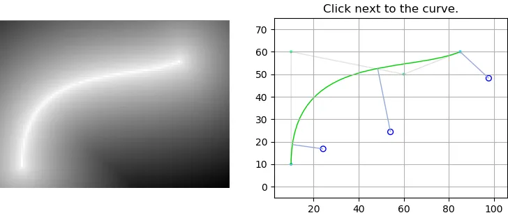
黑色: Bezier曲线,绿色: d(t),紫色: d'(t),红色: d''(t) 找到 d'(t) 的根。我使用了numpy库,该库接受一个多项式的系数作为输入。
numpy库提供Bezier类的Python实现。在我的测试中,这种方法的性能比我的暴力实现(使用样本和细分)快了约三倍。查看交互式示例。
 点击放大。
我使用基本代数来解决这个最小化问题。
点击放大。
我使用基本代数来解决这个最小化问题。
从贝塞尔曲线方程开始。
B(t) = (1 - t)^3 * p0 + 3 * (1 - t)^2 * t * p1 + 3 * (1 - t) * t^2 * p2 + t^3 * p3
由于我正在使用numpy,我的点被表示为numpy向量(矩阵)。这意味着
p0是一维的,例如(1, 4.2)。如果您处理两个浮点变量,则可能需要多个方程(对于x和y):Bx(t) = (1-t)^3*px_0 + ...
将其转换为四个系数的标准形式。

您可以通过扩展原方程式来写出四个系数。


可以使用勾股定理计算点p到曲线B(t)的距离。
在这里,a和b是我们的点 x 和 y 的两个维度。这意味着平方距离 D(t) 是:

我现在不计算平方根,因为只要比较相对平方距离就足够了。所有以下的方程都是关于 平方 距离的。
这个函数 D(t) 描述了图形和点之间的距离。我们感兴趣的是在 t 在 [0, 1] 的范围内的最小值。为了找到它们,我们必须对函数进行两次导数。距离函数的第一阶导数是一个5次多项式:
二阶导数是:

Desmos图表让我们可以查看不同的函数。
D(t) d'(t) = 0 d''(t) >= 0 t
黑色: Bezier曲线,绿色: d(t),紫色: d'(t),红色: d''(t) 找到 d'(t) 的根。我使用了numpy库,该库接受一个多项式的系数作为输入。
dcoeffs = np.stack([da, db, dc, dd, de, df])
roots = np.roots(dcoeffs)
去除虚根(仅保留实根),并删除任何< 0或> 1的根。使用三次贝塞尔曲线,可能还剩下0-3个根。
接下来,对于每个t in roots,检查每个|B(t) - pt|的距离。同时检查B(0)和B(1)的距离,因为贝塞尔曲线的起点和终点可能是最接近的点(尽管它们不是距离函数的局部极小值)。
返回最近的点。
我附上了Python中的Bezier类。请查看github链接以获取使用示例。
import numpy as np

# Bezier Class representing a CUBIC bezier defined by four
# control points.
#
# at(t):            gets a point on the curve at t
# distance2(pt)      returns the closest distance^2 of
#                   pt and the curve
# closest(pt)       returns the point on the curve
#                   which is closest to pt
# maxes(pt)         plots the curve using matplotlib
class Bezier(object):
    exp3 = np.array([[3, 3], [2, 2], [1, 1], [0, 0]], dtype=np.float32)
    exp3_1 = np.array([[[3, 3], [2, 2], [1, 1], [0, 0]]], dtype=np.float32)
    exp4 = np.array([[4], [3], [2], [1], [0]], dtype=np.float32)
    boundaries = np.array([0, 1], dtype=np.float32)

    # Initialize the curve by assigning the control points.
    # Then create the coefficients.
    def __init__(self, points):
        assert isinstance(points, np.ndarray)
        assert points.dtype == np.float32
        self.points = points
        self.create_coefficients()

    # Create the coefficients of the bezier equation, bringing
    # the bezier in the form:
    # f(t) = a * t^3 + b * t^2 + c * t^1 + d
    #
    # The coefficients have the same dimensions as the control
    # points.
    def create_coefficients(self):
        points = self.points
        a = - points[0] + 3*points[1] - 3*points[2] + points[3]
        b = 3*points[0] - 6*points[1] + 3*points[2]
        c = -3*points[0] + 3*points[1]
        d = points[0]
        self.coeffs = np.stack([a, b, c, d]).reshape(-1, 4, 2)

    # Return a point on the curve at the parameter t.
    def at(self, t):
        if type(t) != np.ndarray:
            t = np.array(t)
        pts = self.coeffs * np.power(t, self.exp3_1)
        return np.sum(pts, axis = 1)

    # Return the closest DISTANCE (squared) between the point pt
    # and the curve.
    def distance2(self, pt):
        points, distances, index = self.measure_distance(pt)
        return distances[index]

    # Return the closest POINT between the point pt
    # and the curve.
    def closest(self, pt):
        points, distances, index = self.measure_distance(pt)
        return points[index]

    # Measure the distance^2 and closest point on the curve of
    # the point pt and the curve. This is done in a few steps:
    # 1     Define the distance^2 depending on the pt. I am
    #       using the squared distance because it is sufficient
    #       for comparing distances and doesn't have the over-
    #       head of an additional root operation.
    #       D(t) = (f(t) - pt)^2
    # 2     Get the roots of D'(t). These are the extremes of
    #       D(t) and contain the closest points on the unclipped
    #       curve. Only keep the minima by checking if
    #       D''(roots) > 0 and discard imaginary roots.
    # 3     Calculate the distances of the pt to the minima as
    #       well as the start and end of the curve and return
    #       the index of the shortest distance.
    #
    # This desmos graph is a helpful visualization.
    # https://www.desmos.com/calculator/ktglugn1ya
    def measure_distance(self, pt):
        coeffs = self.coeffs

        # These are the coefficients of the derivatives d/dx and d/(d/dx).
        da = 6*np.sum(coeffs[0][0]*coeffs[0][0])
        db = 10*np.sum(coeffs[0][0]*coeffs[0][1])
        dc = 4*(np.sum(coeffs[0][1]*coeffs[0][1]) + 2*np.sum(coeffs[0][0]*coeffs[0][2]))
        dd = 6*(np.sum(coeffs[0][0]*(coeffs[0][3]-pt)) + np.sum(coeffs[0][1]*coeffs[0][2]))
        de = 2*(np.sum(coeffs[0][2]*coeffs[0][2])) + 4*np.sum(coeffs[0][1]*(coeffs[0][3]-pt))
        df = 2*np.sum(coeffs[0][2]*(coeffs[0][3]-pt))

        dda = 5*da
        ddb = 4*db
        ddc = 3*dc
        ddd = 2*dd
        dde = de
        dcoeffs = np.stack([da, db, dc, dd, de, df])
        ddcoeffs = np.stack([dda, ddb, ddc, ddd, dde]).reshape(-1, 1)

        # Calculate the real extremes, by getting the roots of the first
        # derivativ of the distance function.
        extrema = np_real_roots(dcoeffs)
        # Remove the roots which are out of bounds of the clipped range [0, 1].
        # [future reference] https://stackoverflow.com/questions/47100903/deleting-every-3rd-element-of-a-tensor-in-tensorflow
        dd_clip = (np.sum(ddcoeffs * np.power(extrema, self.exp4)) >= 0) & (extrema > 0) & (extrema < 1)
        minima = extrema[dd_clip]

        # Add the start and end position as possible positions.
        potentials = np.concatenate((minima, self.boundaries))

        # Calculate the points at the possible parameters t and
        # get the index of the closest
        points = self.at(potentials.reshape(-1, 1, 1))
        distances = np.sum(np.square(points - pt), axis = 1)
        index = np.argmin(distances)

        return points, distances, index


    # Point the curve to a matplotlib figure.
    # maxes         ... the axes of a matplotlib figure
    def plot(self, maxes):
        import matplotlib.path as mpath
        import matplotlib.patches as mpatches
        Path = mpath.Path
        pp1 = mpatches.PathPatch(
            Path(self.points, [Path.MOVETO, Path.CURVE4, Path.CURVE4, Path.CURVE4]),
            fc="none")#, transform=ax.transData)
        pp1.set_alpha(1)
        pp1.set_color('#00cc00')
        pp1.set_fill(False)
        pp2 = mpatches.PathPatch(
            Path(self.points, [Path.MOVETO, Path.LINETO , Path.LINETO , Path.LINETO]),
            fc="none")#, transform=ax.transData)
        pp2.set_alpha(0.2)
        pp2.set_color('#666666')
        pp2.set_fill(False)

        maxes.scatter(*zip(*self.points), s=4, c=((0, 0.8, 1, 1), (0, 1, 0.5, 0.8), (0, 1, 0.5, 0.8),
                                                  (0, 0.8, 1, 1)))
        maxes.add_patch(pp2)
        maxes.add_patch(pp1)

# Wrapper around np.roots, but only returning real
# roots and ignoring imaginary results.
def np_real_roots(coefficients, EPSILON=1e-6):
    r = np.roots(coefficients)
    return r.real[abs(r.imag) < EPSILON]
- Leander
2
1贝塞尔曲线方程不正确(在“从贝塞尔曲线方程开始。”之后的那个)。它应该是
B(t) = (1 - t)^3 * p0 + 3 * (1 - t)^2 * t * p1 + 3 * (1 - t) * t^2 * p2 + t^3 * p3。 - Nimble1已经修复。=) - Leander
13
根据您的容忍度,采用暴力方法并接受误差。这种算法在某些罕见情况下可能是错误的,但在大多数情况下,它会找到非常接近正确答案的点,并且结果会随着切片数量的增加而改善。它只是在曲线上沿着规则间隔尝试每个点,并返回找到的最佳点。
public double getClosestPointToCubicBezier(double fx, double fy, int slices, double x0, double y0, double x1, double y1, double x2, double y2, double x3, double y3)  {
    double tick = 1d / (double) slices;
    double x;
    double y;
    double t;
    double best = 0;
    double bestDistance = Double.POSITIVE_INFINITY;
    double currentDistance;
    for (int i = 0; i <= slices; i++) {
        t = i * tick;
        //B(t) = (1-t)**3 p0 + 3(1 - t)**2 t P1 + 3(1-t)t**2 P2 + t**3 P3
        x = (1 - t) * (1 - t) * (1 - t) * x0 + 3 * (1 - t) * (1 - t) * t * x1 + 3 * (1 - t) * t * t * x2 + t * t * t * x3;
        y = (1 - t) * (1 - t) * (1 - t) * y0 + 3 * (1 - t) * (1 - t) * t * y1 + 3 * (1 - t) * t * t * y2 + t * t * t * y3;

        currentDistance = Point.distanceSq(x,y,fx,fy);
        if (currentDistance < bestDistance) {
            bestDistance = currentDistance;
            best = t;
        }
    }
    return best;
}
你可以通过找到最近的点并在该点周围进行递归来获得更好、更快的效果。
public double getClosestPointToCubicBezier(double fx, double fy, int slices, int iterations, double x0, double y0, double x1, double y1, double x2, double y2, double x3, double y3) {
    return getClosestPointToCubicBezier(iterations, fx, fy, 0, 1d, slices, x0, y0, x1, y1, x2, y2, x3, y3);
}

private double getClosestPointToCubicBezier(int iterations, double fx, double fy, double start, double end, int slices, double x0, double y0, double x1, double y1, double x2, double y2, double x3, double y3) {
    if (iterations <= 0) return (start + end) / 2;
    double tick = (end - start) / (double) slices;
    double x, y, dx, dy;
    double best = 0;
    double bestDistance = Double.POSITIVE_INFINITY;
    double currentDistance;
    double t = start;
    while (t <= end) {
        //B(t) = (1-t)**3 p0 + 3(1 - t)**2 t P1 + 3(1-t)t**2 P2 + t**3 P3
        x = (1 - t) * (1 - t) * (1 - t) * x0 + 3 * (1 - t) * (1 - t) * t * x1 + 3 * (1 - t) * t * t * x2 + t * t * t * x3;
        y = (1 - t) * (1 - t) * (1 - t) * y0 + 3 * (1 - t) * (1 - t) * t * y1 + 3 * (1 - t) * t * t * y2 + t * t * t * y3;


        dx = x - fx;
        dy = y - fy;
        dx *= dx;
        dy *= dy;
        currentDistance = dx + dy;
        if (currentDistance < bestDistance) {
            bestDistance = currentDistance;
            best = t;
        }
        t += tick;
    }
    return getClosestPointToCubicBezier(iterations - 1, fx, fy, Math.max(best - tick, 0d), Math.min(best + tick, 1d), slices, x0, y0, x1, y1, x2, y2, x3, y3);
}
在这两种情况下,您都可以轻松地执行四元运算:
x = (1 - t) * (1 - t) * x0 + 2 * (1 - t) * t * x1 + t * t * x2; //quad.
y = (1 - t) * (1 - t) * y0 + 2 * (1 - t) * t * y1 + t * t * y2; //quad.
通过切换方程式。
虽然接受的答案是正确的,你确实可以计算出根并比较那些东西。如果你只需要找到曲线上最近的点,这个方法就可以做到。
关于评论中的Ben。你不能像我对三次和二次形式那样简写几百个控制点范围内的公式。因为每添加一个贝塞尔曲线所需的数量意味着你要为它们构建一个勾股金字塔,我们基本上正在处理越来越庞大的数字字符串。对于二次曲线,你需要1、2、1,对于三次曲线,你需要1、3、3、1。你最终会构建越来越大的金字塔,并最终用Casteljau算法(我为了加快速度写了这个)将其分解:
/**
 * Performs deCasteljau's algorithm for a bezier curve defined by the given control points.
 *
 * A cubic for example requires four points. So it should get at least an array of 8 values
 *
 * @param controlpoints (x,y) coord list of the Bezier curve.
 * @param returnArray Array to store the solved points. (can be null)
 * @param t Amount through the curve we are looking at.
 * @return returnArray
 */
public static float[] deCasteljau(float[] controlpoints, float[] returnArray, float t) {
    int m = controlpoints.length;
    int sizeRequired = (m/2) * ((m/2) + 1);
    if (returnArray == null) returnArray = new float[sizeRequired];
    if (sizeRequired > returnArray.length) returnArray = Arrays.copyOf(controlpoints, sizeRequired); //insure capacity
    else System.arraycopy(controlpoints,0,returnArray,0,controlpoints.length);
    int index = m; //start after the control points.
    int skip = m-2; //skip if first compare is the last control point.
    for (int i = 0, s = returnArray.length - 2; i < s; i+=2) {
        if (i == skip) {
            m = m - 2;
            skip += m;
            continue;
        }
        returnArray[index++] = (t * (returnArray[i + 2] - returnArray[i])) + returnArray[i];
        returnArray[index++] = (t * (returnArray[i + 3] - returnArray[i + 1])) + returnArray[i + 1];
    }
    return returnArray;
}
你需要直接使用算法,不仅用于计算曲线上出现的x、y值,还需要用它执行实际和正确的Bezier细分算法(有其他算法,但我建议使用这个),以计算实际曲线而非像我一样将其分割成线段的近似值。或者说是包含曲线的多边形外壳。
通过在给定t处使用上述算法来对曲线进行细分,例如当T=0.5时将曲线切成两半(注意0.2会将其分为20%和80%)。然后你可以索引金字塔侧面和从基底构建的另一侧的各个点。例如,在三次方程中:
   9
  7 8
 4 5 6
0 1 2 3
您需要将0、1、2、3作为控制点输入算法,然后在0、4、7、9和9、8、6、3处索引两条完美细分的曲线。请注意,这些曲线起点和终点相同,最终索引点9是另一个新锚点。有了这个,您可以完美地细分贝塞尔曲线。
然后要找到最接近的点,您需要不断将曲线细分成不同部分,注意贝塞尔曲线的整个曲线都包含在控制点的凸多边形中。也就是说,如果我们将点0、1、2、3变成连接0、3的封闭路径,则该曲线必须完全位于该多边形凸包内。因此,我们定义给定点P,然后继续细分曲线,直到某个时刻,我们知道一条曲线的最远点比另一条曲线的最近点更接近。我们只需将该点P与所有曲线的控制点和锚点进行比较,并且舍弃任何最近点(无论是锚点还是控制点)距离其他曲线的最远点更远的活动列表中的曲线。然后我们细分所有活动曲线并再次执行此操作。最终,我们会非常细分曲线,每个步骤舍弃约一半(意味着它应该是O(n log n)),直到我们的误差基本可以忽略不计。此时,我们将活动曲线称为最接近点(可能有多个),并且注意到高度细分的曲线中的误差基本相当于一个点。或者只需决定哪个锚点更接近,就是我们点P的最近点。我们知道误差非常具体。
但是,这需要我们实际上拥有一个强大的解决方案,并执行一个确定正确的算法,并正确找到绝对最接近我们点的微小部分。而且它仍然应该相对较快。
- Tatarize
4
1这是如何工作的?
fx和fy代表什么?为什么恰好有4个其他的x/y坐标,而不多也不少?我如何将其应用于具有数百个点的任意贝塞尔曲线? - Ky -2基本上是因为 Bezout 定理。在高阶中有一些有点棘手的部分。就像在基本定理代数中,贝塞尔曲线有多少个根(可能会改变给定方向),就有多少个属性。问题直接要求一个三次贝塞尔曲线,这是一个很好的近似,但如果你想要更高阶的曲线,你需要找到一些在数学上能够确保在某些范围内产生正确答案的东西。fx,fy,找到x,找到y。 - Tatarize
2@BenLeggiero,更新了答案以解释如何完整且正确地执行此操作。此外,您可以简单地应用Decasteljau算法,在曲线上找到一些良好的锚点,并以二进制搜索方式在其中跳动。但是,我不确定这是否是一个好的答案。虽然我确信它在相当低的阶数下会工作得相当好。 - Tatarize
1非常感谢您额外的工作和信息,太棒了 :) - Ky -
1
这个问题的解决方法是获取贝塞尔曲线上的所有可能点并比较每一个距离。点的数量可以通过控制“detail”变量来实现。
下面是使用Unity(C#)实现的代码:
请注意,Bezier类只包含4个点。
这可能不是最好的方法,因为它可能会根据细节变得非常缓慢。
下面是使用Unity(C#)实现的代码:
public Vector2 FindNearestPointOnBezier(Bezier bezier, Vector2 point)
{
    float detail = 100;
    List<Vector2> points = new List<Vector2>();

    for (float t = 0; t < 1f; t += 1f / detail)
    {
        // this function can be exchanged for any bezier curve
        points.Add(Functions.CalculateBezier(bezier.a, bezier.b, bezier.c, bezier.d, t));
    }

    Vector2 closest = Vector2.zero;
    float minDist = Mathf.Infinity;

    foreach (Vector2 p in points)
    {
        // use sqrMagnitude as it is faster
        float dist = (p - point).sqrMagnitude;

        if (dist < minDist)
        {
            minDist = dist;
            closest = p;
        }
    }

    return closest;
}
请注意,Bezier类只包含4个点。
这可能不是最好的方法,因为它可能会根据细节变得非常缓慢。
- timeBenter
网页内容由stack overflow 提供, 点击上面的可以查看英文原文,
原文链接
原文链接