np.einsum 是如何工作的?
给定数组 A 和 B,它们的矩阵乘法加上转置可以使用 (A @ B).T 或等效地使用以下方式计算:
np.einsum("ij, jk -> ki", A, B)
np.einsum 是如何工作的?
给定数组 A 和 B,它们的矩阵乘法加上转置可以使用 (A @ B).T 或等效地使用以下方式计算:
np.einsum("ij, jk -> ki", A, B)
假设我们有两个多维数组,`A`和`B`。现在假设我们想要...
使用`einsum`比使用NumPy函数(例如`multiply`、`sum`和`transpose`)的组合更快且更节省内存。
这里是一个简单(但不完全琐碎)的例子。取以下两个数组:
A = np.array([0, 1, 2])

B = np.array([[ 0,  1,  2,  3],
              [ 4,  5,  6,  7],
              [ 8,  9, 10, 11]])
A和B进行逐元素相乘,然后沿新数组的行进行求和。在“普通”NumPy中,我们会这样写:
```python
np.sum(A * B, axis=1)
```>>> (A[:, np.newaxis] * B).sum(axis=1)
array([ 0, 22, 76])
因此,在这里,对 A 的索引操作将两个数组的第一个轴排成一行,以便进行广播乘法。然后将产品数组的行相加以返回答案。
现在,如果我们想使用 einsum,我们可以写成:
>>> np.einsum('i,ij->i', A, B)
array([ 0, 22, 76])
signature字符串'i,ij->i'是关键,需要一点解释。您可以将其分为两半。在左侧(->左侧)我们标记了两个输入数组。在->右侧,我们标记了我们想要得到的数组。
接下来会发生以下情况:
A只有一个轴,我们将其标记为i。而B有两个轴,我们将轴0标记为i,将轴1标记为j。
通过在两个输入数组中重复标签i,我们告诉einsum这两个轴应该相乘。换句话说,我们正在将数组A与数组B的每一列相乘,就像A [:,np.newaxis] * B一样。
请注意,在我们想要的输出中,j不出现作为标签;我们只使用了i(我们希望最终得到一个1D数组)。通过省略该标签,我们告诉einsum在此轴上求和。换句话说,我们正在对产品的行求和,就像.sum(axis=1)一样。
einsum所需了解的全部内容。建议多试一下;如果输出中保留两个标签'i,ij->ij',将得到一个二维数组的积(与A[:, np.newaxis] * B相同)。如果不指定输出标签'i,ij->,将得到一个单一数字的积(与(A[:, np.newaxis] * B).sum()相同)。einsum的优点在于它不会先构建一个临时的乘积数组;它会边计算边求和。这可以大大节省内存的使用。A = array([[1, 1, 1],
[2, 2, 2],
[5, 5, 5]])
B = array([[0, 1, 0],
[1, 1, 0],
[1, 1, 1]])
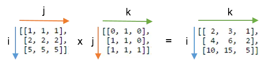
np.einsum('ij,jk->ik', A, B)计算点积。下面是一张展示了A和B的标签以及函数输出数组的图片:
j被重复使用了 - 这意味着我们正在将A的行与B的列相乘。此外,标签j没有包含在输出中 - 我们正在对这些乘积求和。标签i和k保留在输出中,因此我们得到一个二维数组。j未被求和的数组进行比较。下面,在左侧您可以看到从编写np.einsum('ij,jk->ijk', A, B)(即我们保留了标签j)而得到的三维数组。
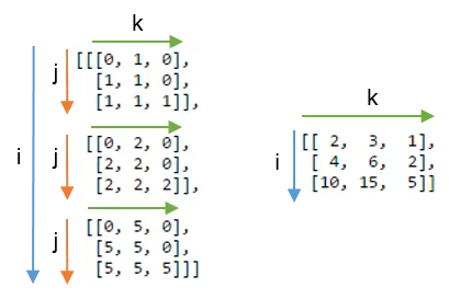
对于轴j的求和给出了预期的点积,如右侧所示。
为了更好地理解einsum,使用下标符号实现熟悉的NumPy数组操作可能会很有用。任何涉及组合乘法和轴求和的操作都可以使用einsum来编写。
设A和B是两个长度相同的1D数组。例如,A = np.arange(10)和B = np.arange(5, 15)。
The sum of A can be written:
np.einsum('i->', A)
Element-wise multiplication, A * B, can be written:
np.einsum('i,i->i', A, B)
The inner product or dot product, np.inner(A, B) or np.dot(A, B), can be written:
np.einsum('i,i->', A, B) # or just use 'i,i'
The outer product, np.outer(A, B), can be written:
np.einsum('i,j->ij', A, B)
对于二维数组C和D,前提是它们的轴具有兼容长度(长度相同或其中一个长度为1),以下是一些示例:
The trace of C (sum of main diagonal), np.trace(C), can be written:
np.einsum('ii', C)
Element-wise multiplication of C and the transpose of D, C * D.T, can be written:
np.einsum('ij,ji->ij', C, D)
Multiplying each element of C by the array D (to make a 4D array), C[:, :, None, None] * D, can be written:
np.einsum('ij,kl->ijkl', C, D)
numpy.einsum() 的概念非常容易,只要你能直观理解它。举个例子,我们从描述矩阵乘法的简单说明开始。
numpy.einsum(),你只需要将所谓的 下标字符串 作为参数传递,然后跟上你的 输入数组。
假设你有两个二维数组 A 和B,你想进行矩阵乘法。那么,你只需要执行以下操作:np.einsum("ij, jk -> ik", A, B)
这里的下标字符串ij对应于数组A,而下标字符串jk对应于数组B。此外,这里最重要的一点是,每个下标字符串中的字符数必须与数组的维度匹配(即,2D数组为两个字符,3D数组为三个字符,以此类推)。如果在下标字符串之间重复字符(在我们的例子中为j),则表示您希望在这些维度上执行einsum。因此,它们将被求和(即该维度将被消去)。
在->符号后面的下标字符串表示我们结果数组的维度。
如果将其留空,则将对所有元素求和并返回标量值作为结果。否则,结果数组的维度将根据下标字符串确定。在我们的例子中,它将是ik。这很直观,因为我们知道矩阵乘法需要数组A中的列数与数组B中的行数匹配,这正是此处所发生的(即通过在下标字符串中重复字符j来编码此信息)。
以下是一些示例,展示了np.einsum()在实现一些常见的张量或nd-array操作时的使用/功能。
输入
# a vector
In [197]: vec
Out[197]: array([0, 1, 2, 3])

# an array
In [198]: A
Out[198]:
array([[11, 12, 13, 14],
       [21, 22, 23, 24],
       [31, 32, 33, 34],
       [41, 42, 43, 44]])

# another array
In [199]: B
Out[199]:
array([[1, 1, 1, 1],
       [2, 2, 2, 2],
       [3, 3, 3, 3],
       [4, 4, 4, 4]])
1) 矩阵乘法(类似于 np.matmul(arr1, arr2))
In [200]: np.einsum("ij, jk -> ik", A, B)
Out[200]:
array([[130, 130, 130, 130],
       [230, 230, 230, 230],
       [330, 330, 330, 330],
       [430, 430, 430, 430]])
2) 提取沿主对角线的元素(类似于 np.diag(arr))
In [202]: np.einsum("ii -> i", A)
Out[202]: array([11, 22, 33, 44])
3) Hadamard乘积(即两个数组的逐元素相乘)(类似于arr1 * arr2)
In [203]: np.einsum("ij, ij -> ij", A, B)
Out[203]:
array([[ 11,  12,  13,  14],
       [ 42,  44,  46,  48],
       [ 93,  96,  99, 102],
       [164, 168, 172, 176]])
4) 逐元素平方(类似于np.square(arr)或arr ** 2)
In [210]: np.einsum("ij, ij -> ij", B, B)
Out[210]:
array([[ 1,  1,  1,  1],
       [ 4,  4,  4,  4],
       [ 9,  9,  9,  9],
       [16, 16, 16, 16]])
5) 跟踪(即主对角线元素的总和)(类似于np.trace(arr))
In [217]: np.einsum("ii -> ", A)
Out[217]: 110
6) 矩阵转置(类似于 np.transpose(arr))
In [221]: np.einsum("ij -> ji", A)
Out[221]:
array([[11, 21, 31, 41],
       [12, 22, 32, 42],
       [13, 23, 33, 43],
       [14, 24, 34, 44]])
7) 外积(向量的) (类似于 np.outer(vec1, vec2))
In [255]: np.einsum("i, j -> ij", vec, vec)
Out[255]:
array([[0, 0, 0, 0],
       [0, 1, 2, 3],
       [0, 2, 4, 6],
       [0, 3, 6, 9]])
8) 向量内积 (Inner Product) (类似于 np.inner(vec1, vec2))
In [256]: np.einsum("i, i -> ", vec, vec)
Out[256]: 14
9) 沿轴0求和(类似于 np.sum(arr, axis=0))
In [260]: np.einsum("ij -> j", B)
Out[260]: array([10, 10, 10, 10])
10) 沿轴1求和(类似于np.sum(arr, axis=1))
In [261]: np.einsum("ij -> i", B)
Out[261]: array([ 4,  8, 12, 16])
11) 批量矩阵乘法
In [287]: BM = np.stack((A, B), axis=0)

In [288]: BM
Out[288]:
array([[[11, 12, 13, 14],
        [21, 22, 23, 24],
        [31, 32, 33, 34],
        [41, 42, 43, 44]],

       [[ 1,  1,  1,  1],
        [ 2,  2,  2,  2],
        [ 3,  3,  3,  3],
        [ 4,  4,  4,  4]]])

In [289]: BM.shape
Out[289]: (2, 4, 4)

# batch matrix multiply using einsum
In [292]: BMM = np.einsum("bij, bjk -> bik", BM, BM)

In [293]: BMM
Out[293]:
array([[[1350, 1400, 1450, 1500],
        [2390, 2480, 2570, 2660],
        [3430, 3560, 3690, 3820],
        [4470, 4640, 4810, 4980]],

       [[  10,   10,   10,   10],
        [  20,   20,   20,   20],
        [  30,   30,   30,   30],
        [  40,   40,   40,   40]]])

In [294]: BMM.shape
Out[294]: (2, 4, 4)
12) 沿第二轴求和(类似于 np.sum(arr, axis=2))
In [330]: np.einsum("ijk -> ij", BM)
Out[330]:
array([[ 50,  90, 130, 170],
       [  4,   8,  12,  16]])
13) 对数组中的所有元素求和(类似于 np.sum(arr))
In [335]: np.einsum("ijk -> ", BM)
Out[335]: 480
14) 多轴求和(即边缘化)
(类似于np.sum(arr, axis=(axis0, axis1, axis2, axis3, axis4, axis6, axis7)))
# 8D array
In [354]: R = np.random.standard_normal((3,5,4,6,8,2,7,9))

# marginalize out axis 5 (i.e. "n" here)
In [363]: esum = np.einsum("ijklmnop -> n", R)

# marginalize out axis 5 (i.e. sum over rest of the axes)
In [364]: nsum = np.sum(R, axis=(0,1,2,3,4,6,7))

In [365]: np.allclose(esum, nsum)
Out[365]: True
15) 双点积(类似于np.sum(hadamard-product),参见3)
In [772]: A
Out[772]:
array([[1, 2, 3],
       [4, 2, 2],
       [2, 3, 4]])

In [773]: B
Out[773]:
array([[1, 4, 7],
       [2, 5, 8],
       [3, 6, 9]])

In [774]: np.einsum("ij, ij -> ", A, B)
Out[774]: 124
16) 2D和3D数组相乘
在解决线性方程组(Ax = b)并验证结果时,这种乘法非常有用。
# inputs
In [115]: A = np.random.rand(3,3)
In [116]: b = np.random.rand(3, 4, 5)

# solve for x
In [117]: x = np.linalg.solve(A, b.reshape(b.shape[0], -1)).reshape(b.shape)

# 2D and 3D array multiplication :)
In [118]: Ax = np.einsum('ij, jkl', A, x)

# indeed the same!
In [119]: np.allclose(Ax, b)
Out[119]: True
相反地,如果我们必须使用np.matmul()进行验证,我们需要执行几个reshape操作才能获得相同的结果,例如:
# reshape 3D array `x` to 2D, perform matmul
# then reshape the resultant array to 3D
In [123]: Ax_matmul = np.matmul(A, x.reshape(x.shape[0], -1)).reshape(x.shape)

# indeed correct!
In [124]: np.allclose(Ax, Ax_matmul)
Out[124]: True
当阅读einsum方程时,我发现将它们简化为其必要版本最有帮助。
让我们从以下(令人印象深刻的)声明开始:
C = np.einsum('bhwi,bhwj->bij', A, B)
首先,我们看到在箭头之前有两个由逗号分隔的4字母块 - bhwi和bhwj,以及一个单独的3字母块bij。因此,该方程从两个秩为4的张量输入产生秩为3的张量结果。
现在,让我们将每个块中的每个字母视为范围变量的名称。字母出现的位置是它在张量中覆盖的轴的索引。因此,产生C的每个元素的命令式求和必须从三个嵌套的for循环开始,每个循环对应C的一个索引。
for b in range(...):
    for i in range(...):
        for j in range(...):
            # the variables b, i and j index C in the order of their appearance in the equation
            C[b, i, j] = ...
for循环。我们现在将保留范围未确定。h和w。 为每个这样的变量添加一个内部嵌套的for循环:for b in range(...):
for i in range(...):
for j in range(...):
C[b, i, j] = 0
for h in range(...):
for w in range(...):
...
在最内层循环中,我们已经定义了所有的索引,因此我们可以编写实际的求和公式,翻译完成:
# three nested for-loops that index the elements of C
for b in range(...):
    for i in range(...):
        for j in range(...):

            # prepare to sum
            C[b, i, j] = 0

            # two nested for-loops for the two indexes that don't appear on the right-hand side
            for h in range(...):
                for w in range(...):
                    # Sum! Compare the statement below with the original einsum formula
                    # 'bhwi,bhwj->bij'

                    C[b, i, j] += A[b, h, w, i] * B[b, h, w, j]
# C's shape is determined by the shapes of the inputs
# b indexes both A and B, so its range can come from either A.shape or B.shape
# i indexes only A, so its range can only come from A.shape, the same is true for j and B
assert A.shape[0] == B.shape[0]
assert A.shape[1] == B.shape[1]
assert A.shape[2] == B.shape[2]
C = np.zeros((A.shape[0], A.shape[3], B.shape[3]))
for b in range(A.shape[0]): # b indexes both A and B, or B.shape[0], which must be the same
    for i in range(A.shape[3]):
        for j in range(B.shape[3]):
            # h and w can come from either A or B
            for h in range(A.shape[1]):
                for w in range(A.shape[2]):
                    C[b, i, j] += A[b, h, w, i] * B[b, h, w, j]
np.einsum的看法大多数回答都是通过示例来解释,我想提供一个额外的观点。
您可以将einsum视为广义矩阵求和运算符。给定的字符串包含表示轴的标签。我喜欢把它看作您的操作定义。下标提供了两个明显的约束条件:
每个输入数组的轴数,
输入之间轴大小的相等性。
让我们以最初的示例为例:np.einsum('ij,jk->ki', A, B)。这里的约束条件 1. 转化为 A.ndim == 2 和 B.ndim == 2,而 2. 转化为 A.shape[1] == B.shape[0]。
正如您稍后将看到的那样,还有其他约束条件。例如:
输出下标中的标签不能出现超过一次。
输出下标中的标签必须出现在输入下标中。
当查看ij,jk->ki时,您可以将其视为:
哪些来自输入数组的组件将对输出数组的组件
[k,i]做出贡献。
下标包含每个输出数组组件的操作的确切定义。
我们将坚持使用操作ij,jk->ki,以及以下对A和B的定义:
>>> A = np.array([[1,4,1,7], [8,1,2,2], [7,4,3,4]])
>>> A.shape
(3, 4)

>>> B = np.array([[2,5], [0,1], [5,7], [9,2]])
>>> B.shape
(4, 2)
Z 的形状为 (B.shape[1], A.shape[0]),可以通过以下方式进行简单构造。首先创建一个空数组作为 Z:Z = np.zeros((B.shape[1], A.shape[0]))
for i in range(A.shape[0]):
for j in range(A.shape[1]):
for k range(B.shape[0]):
Z[k, i] += A[i, j]*B[j, k] # ki <- ij*jk
np.einsum是用于在输出数组中累加贡献的。每个(A[i,j], B[j,k])对都被视为对每个Z[k, i]元素的贡献。
你可能已经注意到,它看起来与计算一般矩阵乘法非常相似...
这是Python中np.einsum的最小实现。这应该有助于理解底层发生了什么。
随着我们的学习,我会不断参考之前的例子。将 inputs 定义为 [A, B]。
np.einsum实际上可以接受多于两个的输入。在接下来的内容中,我们将关注一般情况:n个输入和n个输入下标。主要目标是找到迭代的域,即所有范围的笛卡尔积。
我们无法依靠手动编写for循环,因为我们不知道会有多少个。主要思想是:我们需要找到所有唯一的标签(我将使用key和keys来引用它们),找到相应的数组形状,然后为每个标签创建范围,并使用itertools.product计算范围的乘积以获得研究域。
| 索引 | 键值 |
约束条件 | 大小 |
范围 |
|---|---|---|---|---|
| 1 | 'i' |
A.shape[0] |
3 | range(0, 3) |
| 2 | 'j' |
A.shape[1] == B.shape[0] |
4 | range(0, 4) |
| 0 | 'k' |
B.shape[1] |
2 | range(0, 2) |
研究领域是笛卡尔积:range(0, 2) x range(0, 3) x range(0, 4)。
Subscripts processing:
>>> expr = 'ij,jk->ki'
>>> qry_expr, res_expr = expr.split('->')
>>> inputs_expr = qry_expr.split(',')
>>> inputs_expr, res_expr
(['ij', 'jk'], 'ki')
Find the unique keys (labels) in the input subscripts:
>>> keys = set([(key, size) for keys, input in zip(inputs_expr, inputs)
               for key, size in list(zip(keys, input.shape))])
{('i', 3), ('j', 4), ('k', 2)}
We should be checking for constraints (as well as in the output subscript)! Using set is a bad idea but it will work for the purpose of this example.
Get the associated sizes (used to initialize the output array) and construct the ranges (used to create our domain of iteration):
>>> sizes = dict(keys)
{'i': 3, 'j': 4, 'k': 2}

>>> ranges = [range(size) for _, size in keys]
[range(0, 2), range(0, 3), range(0, 4)]
We need an list containing the keys (labels):
>>> to_key = sizes.keys()
['k', 'i', 'j']
Compute the cartesian product of the ranges
>>> domain = product(*ranges)
Note: [itertools.product][1] returns an iterator which gets consumed over time.
Initialize the output tensor as:
>>> res = np.zeros([sizes[key] for key in res_expr])
We will be looping over domain:
>>> for indices in domain:
...     pass
For each iteration, indices will contain the values on each axis. In our example, that would provide i, j, and k as a tuple: (k, i, j). For each input (A and B) we need to determine which component to fetch. That's A[i, j] and B[j, k], yes! However, we don't have variables i, j, and k, literally speaking.
We can zip indices with to_key to create a mapping between each key (label) and its current value:
>>> vals = dict(zip(to_key, indices))
To get the coordinates for the output array, we use vals and loop over the keys: [vals[key] for key in res_expr]. However, to use these to index the output array, we need to wrap it with tuple and zip to separate the indices along each axis:
>>> res_ind = tuple(zip([vals[key] for key in res_expr]))
Same for the input indices (although there can be several):
>>> inputs_ind = [tuple(zip([vals[key] for key in expr])) for expr in inputs_expr]
We will use a itertools.reduce to compute the product of all contributing components:
>>> def reduce_mult(L):
...     return reduce(lambda x, y: x*y, L)
Overall the loop over the domain looks like:
>>> for indices in domain:
...     vals = {k: v for v, k in zip(indices, to_key)}
...     res_ind = tuple(zip([vals[key] for key in res_expr]))
...     inputs_ind = [tuple(zip([vals[key] for key in expr]))
...                     for expr in inputs_expr]
...
...     res[res_ind] += reduce_mult([M[i] for M, i in zip(inputs, inputs_ind)])
>>> res
array([[70., 44., 65.],
       [30., 59., 68.]])
这就很接近于np.einsum('ij,jk->ki', A, B)的返回值了!
import numpy as np

>>> a
array([[1, 1, 1],
       [2, 2, 2],
       [3, 3, 3]])
>>> b
array([[0, 1, 2],
       [3, 4, 5],
       [6, 7, 8]])
>>> d = np.einsum('ij, jk->ki', a, b)
注意有三个轴,i、j、k,而且 j 被重复了(在左侧)。i,j 表示 a 的行和列。j,k 表示 b 的行和列。
为了计算乘积并对齐 j 轴,我们需要给 a 添加一个轴。(b 将沿着第一个轴广播)
a[i, j, k]
   b[j, k]

>>> c = a[:,:,np.newaxis] * b
>>> c
array([[[ 0,  1,  2],
        [ 3,  4,  5],
        [ 6,  7,  8]],

       [[ 0,  2,  4],
        [ 6,  8, 10],
        [12, 14, 16]],

       [[ 0,  3,  6],
        [ 9, 12, 15],
        [18, 21, 24]]])
j 在右边没有出现,因此我们对 3x3x3 数组的第二个轴 j 进行求和。
>>> c = c.sum(1)
>>> c
array([[ 9, 12, 15],
       [18, 24, 30],
       [27, 36, 45]])
>>> c.T
array([[ 9, 18, 27],
       [12, 24, 36],
       [15, 30, 45]])

>>> np.einsum('ij, jk->ki', a, b)
array([[ 9, 18, 27],
       [12, 24, 36],
       [15, 30, 45]])
>>>
In [43]: A=np.arange(6).reshape(2,3)
Out[43]:
array([[0, 1, 2],
       [3, 4, 5]])


In [44]: B=np.arange(12).reshape(3,4)
Out[44]:
array([[ 0,  1,  2,  3],
       [ 4,  5,  6,  7],
       [ 8,  9, 10, 11]])
i是A的第一维,C的最后一维;k是B的最后一维,C的第一维。在求和中,“消耗”了j。In [45]: C=np.einsum('ij,jk->ki',A,B)
Out[45]:
array([[20, 56],
[23, 68],
[26, 80],
[29, 92]])
这与np.dot(A,B).T相同 - 它是最终输出的转置。
如果要查看更多关于j的信息,请将C下标更改为ijk:
In [46]: np.einsum('ij,jk->ijk',A,B)
Out[46]:
array([[[ 0,  0,  0,  0],
        [ 4,  5,  6,  7],
        [16, 18, 20, 22]],

       [[ 0,  3,  6,  9],
        [16, 20, 24, 28],
        [40, 45, 50, 55]]])
这也可以用以下方式生成:
A[:,:,None]*B[None,:,:]
即在A的末尾添加一个k维度,在B的前面添加一个i,得到一个(2,3,4)数组。
0 + 4 + 16 = 20,9 + 28 + 55 = 92等;对j求和并转置以获得先前的结果:
np.sum(A[:,:,None] * B[None,:,:], axis=1).T

# C[k,i] = sum(j) A[i,j (,k) ] * B[(i,)  j,k]
-> is easy. Therefore, focus on:
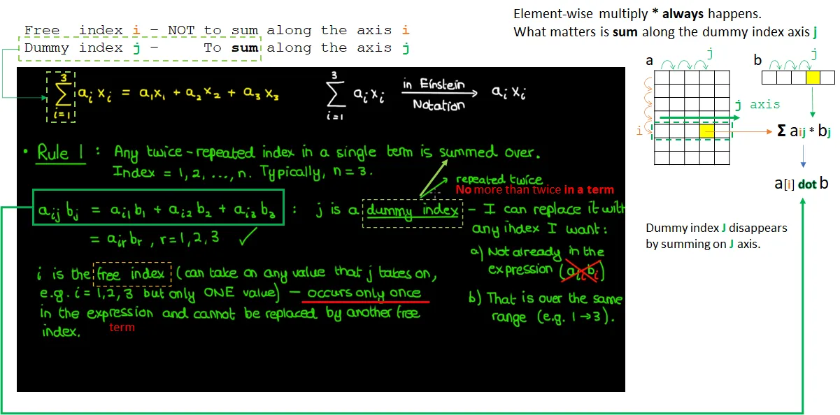
j in np.einsum("ij,jk->ki", a, b)jeinsum("...", a, b), element-wise multiplication always occurs between matrices a and b, regardless of whether there are common indices or not. We can have einsum('xy,wz', a, b), which has no common index in the subscripts 'xy,wz'.j in "ij,jk->ki", then it is called a dummy index in Einstein Summation.
被求和的指标称为求和指标,本例中为“i”。它也被称为哑指标,因为任何符号都可以替换“i”,只要它不与同一项中的指标符号冲突即可。
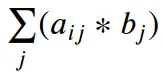
对于图表中绿色方框中的np.einsum("ij,j", a, b),j是哑指标。元素间的乘法 a[i][j] * b[j] 沿着 j 轴求和,得到 Σ ( a[i][j] * b[j] )。
np.inner(a[i], b)。 在这里,具体使用np.inner()并避免np.dot,因为它不是严格的数学点积运算。
假索引可以出现在任何地方,只要符合规则(详见youtube)。
对于np.einsum("ik,il", a, b)中的虚拟索引i,它是矩阵a和b的行索引,因此从a和b中提取一行和一列来生成点积。
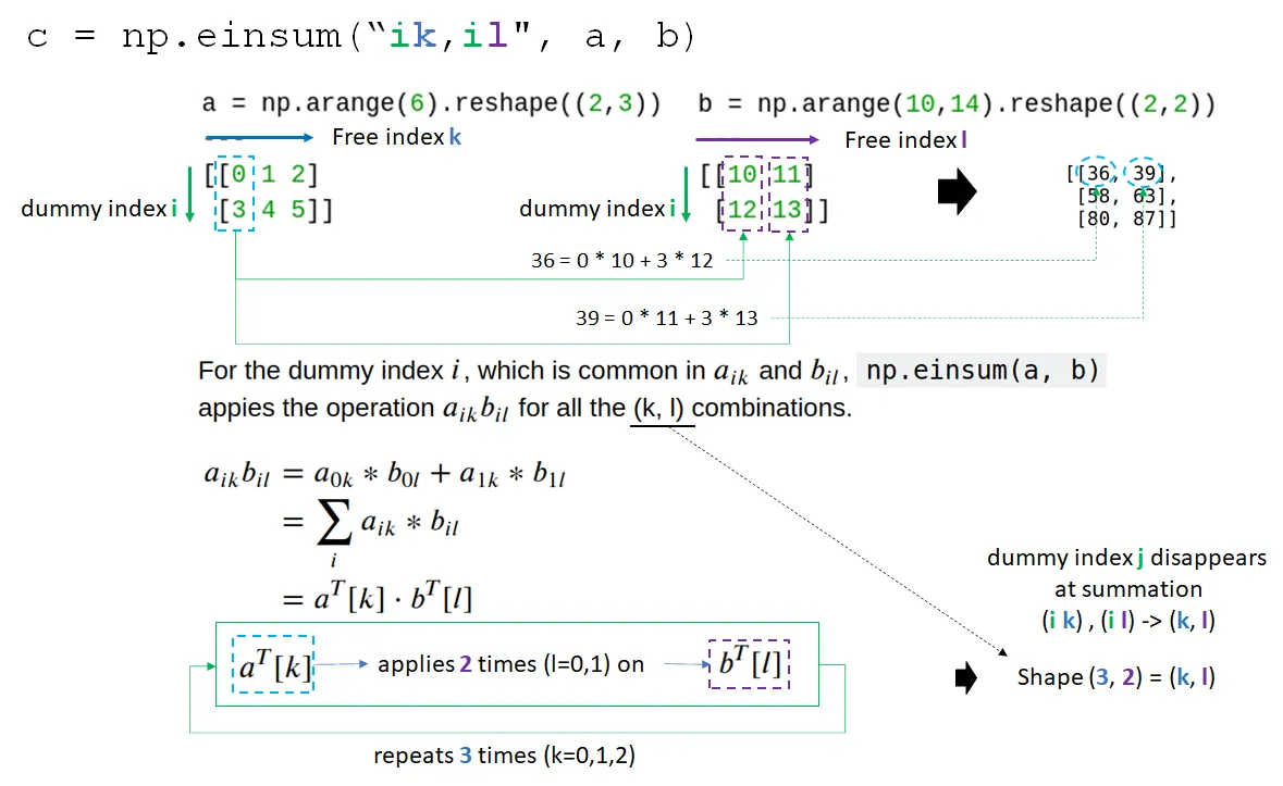
由于求和沿着虚拟索引进行,因此结果矩阵中的虚拟索引消失,因此从"ik,il"中删除了i,形成了形状为(k,l)的矩阵。我们可以通过输出下标标签和->标识符告诉np.einsum("... -> <shape>")指定输出形式。
详见numpy.einsum中的显式模式。
在显式模式下,可以通过指定输出下标标签来直接控制输出。这需要使用标识符
'->'以及输出下标标签列表。此功能增加了函数的灵活性,因为可以在需要时禁用或强制求和。调用np.einsum('i->', a)相当于np.sum(a, axis=-1),而np.einsum('ii->i', a)相当于np.diag(a)。不同之处在于,einsum默认情况下不允许广播。此外,np.einsum('ij,jh->ih', a, b)直接指定了输出下标标签的顺序,因此返回矩阵乘法,与上面隐式模式的示例不同。
一个没有虚拟指数的einsum示例。
"ij")选择每个数组中的一个元素。a的形状为(2,3),每个元素都应用于形状为(2,2)的b。因此,它创建了一个形状为(2,3,2,2)的矩阵,没有任何求和,因为(i,j),(k.l)都是自由指标。
# --------------------------------------------------------------------------------
# For np.einsum("ij,kl", a, b)
# 1-1: Term "ij" or (i,j), two free indices, selects selects an element a[i][j].
# 1-2: Term "kl" or (k,l), two free indices, selects selects an element b[k][l].
# 2:   Each a[i][j] is applied on b[k][l] for element-wise multiplication a[i][j] * b[k,l]
# --------------------------------------------------------------------------------
# for (i,j) in a:
#    for(k,l) in b:
#        a[i][j] * b[k][l]
np.einsum("ij,kl", a, b)

array([[[[ 0,  0],
         [ 0,  0]],

        [[10, 11],
         [12, 13]],

        [[20, 22],
         [24, 26]]],


       [[[30, 33],
         [36, 39]],

        [[40, 44],
         [48, 52]],

        [[50, 55],
         [60, 65]]]])
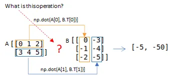
A = np.matrix('0 1 2; 3 4 5')
B = np.matrix('0 -3; -1 -4; -2 -5');
np.einsum('ij,ji->i', A, B)

# Same with
np.diagonal(np.matmul(A,B))
(A*B).diagonal()
---
[ -5 -50]
[ -5 -50]
[[ -5 -50]]
我认为最简单的例子在tensorflow文档中。
将方程转换为einsum符号有四个步骤。让我们以这个方程为例C[i,k] = sum_j A[i,j] * B[j,k]
ik = sum_j ij * jksum_j项,因为它是隐含的。我们得到ik = ij * jk,替换*。我们得到ik = ij, jk->符号分隔。我们得到ij, jk -> ikeinsum解释器只是按相反顺序运行这4个步骤。结果中缺少的所有索引都会被求和。
以下是来自文档的更多示例
# Matrix multiplication
einsum('ij,jk->ik', m0, m1)  # output[i,k] = sum_j m0[i,j] * m1[j, k]

# Dot product
einsum('i,i->', u, v)  # output = sum_i u[i]*v[i]

# Outer product
einsum('i,j->ij', u, v)  # output[i,j] = u[i]*v[j]

# Transpose
einsum('ij->ji', m)  # output[j,i] = m[i,j]

# Trace
einsum('ii', m)  # output[j,i] = trace(m) = sum_i m[i, i]

# Batch matrix multiplication
einsum('aij,ajk->aik', s, t)  # out[a,i,k] = sum_j s[a,i,j] * t[a, j, k]
ij,jk可以自行工作(无需箭头)以形成矩阵乘法。但是为了清晰起见,最好先放置箭头,然后再放置输出维度。这在博客文章中有提到。 - ComputerScientistA的长度为3,与B中的列的长度相同(而B的行的长度为4,无法逐元素地与A相乘)。 - Alex Riley->会影响语义:“在隐式模式下,所选的下标非常重要,因为输出的轴按字母顺序重新排序。这意味着np.einsum('ij', a)不会影响二维数组,而np.einsum('ji', a)会取其转置。” - BallpointBen