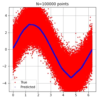
我正在尝试使用Keras和TensorFlow构建一个简单的回归模型。在我的问题中,我的数据以(x, y)的形式存在,其中x和y都是数字。我想建立一个Keras模型来预测y,使用x作为输入。
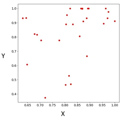
由于我认为图像更能说明问题,这是我的数据:
我的Keras模型如下(数据分为30%测试
注意:
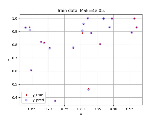
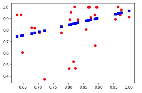
绘制预测结果(蓝色方块为预测值
有人有关于如何复现过度拟合的想法吗?
这是我想要得到的结果: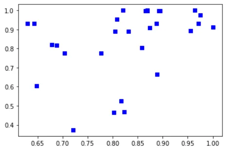 (红点在蓝色正方形下面!)
编辑:
这里提供了上述示例中使用的数据:您可以直接将其复制粘贴到Python解释器中:
由于我认为图像更能说明问题,这是我的数据:
我的Keras模型如下(数据分为30%测试
(X_test,y_test)和70%训练(X_train,y_train)):model = tf.keras.Sequential()
model.add(tf.keras.layers.Dense(32, input_shape=() activation="relu", name="first_layer"))
model.add(tf.keras.layers.Dense(16, activation="relu", name="second_layer"))
model.add(tf.keras.layers.Dense(1, name="output_layer"))
model.compile(loss = "mean_squared_error", optimizer = "adam", metrics=["mse"] )
history = model.fit(X_train, y_train, epochs=500, batch_size=1, verbose=0, shuffle=False)
eval_result = model.evaluate(X_test, y_test)
print("\n\nTest loss:", eval_result, "\n")
predict_Y = model.predict(X)
注意:
X 包含了 X_test 和 X_train。绘制预测结果(蓝色方块为预测值
predict_Y)。
有人有关于如何复现过度拟合的想法吗?
这是我想要得到的结果:
(红点在蓝色正方形下面!)编辑:
这里提供了上述示例中使用的数据:您可以直接将其复制粘贴到Python解释器中:
X_train = [0.704619794270697, 0.6779457393024553, 0.8207082120250023, 0.8588819357831449, 0.8692320257603844, 0.6878750931810429, 0.9556331888763945, 0.77677964510883, 0.7211381534179618, 0.6438319113259414, 0.6478339581502052, 0.9710222750072649, 0.8952188423349681, 0.6303124926673513, 0.9640316662124185, 0.869691568491902, 0.8320164648420931, 0.8236399177660375, 0.8877334038470911, 0.8084042532069621, 0.8045680821762038]
y_train = [0.7766424210611557, 0.8210846773655833, 0.9996114311913593, 0.8041331063189883, 0.9980525368790883, 0.8164056182686034, 0.8925487603333683, 0.7758207470960685, 0.37345286573743475, 0.9325789202459493, 0.6060269037514895, 0.9319771743389491, 0.9990691225991941, 0.9320002808310418, 0.9992560731072977, 0.9980241561997089, 0.8882905258641204, 0.4678339275898943, 0.9312152374846061, 0.9542371205095945, 0.8885893668675711]
X_test = [0.9749191829308574, 0.8735366740730178, 0.8882783211709133, 0.8022891400991644, 0.8650601322313454, 0.8697902997857514, 1.0, 0.8165876695985228, 0.8923841531760973]
y_test = [0.975653685270635, 0.9096752789481569, 0.6653736469114154, 0.46367666660348744, 0.9991817903431941, 1.0, 0.9111205717076893, 0.5264993912088891, 0.9989199241685126]
X = [0.704619794270697, 0.77677964510883, 0.7211381534179618, 0.6478339581502052, 0.6779457393024553, 0.8588819357831449, 0.8045680821762038, 0.8320164648420931, 0.8650601322313454, 0.8697902997857514, 0.8236399177660375, 0.6878750931810429, 0.8923841531760973, 0.8692320257603844, 0.8877334038470911, 0.8735366740730178, 0.8207082120250023, 0.8022891400991644, 0.6303124926673513, 0.8084042532069621, 0.869691568491902, 0.9710222750072649, 0.9556331888763945, 0.8882783211709133, 0.8165876695985228, 0.6438319113259414, 0.8952188423349681, 0.9749191829308574, 1.0, 0.9640316662124185]
Y = [0.7766424210611557, 0.7758207470960685, 0.37345286573743475, 0.6060269037514895, 0.8210846773655833, 0.8041331063189883, 0.8885893668675711, 0.8882905258641204, 0.9991817903431941, 1.0, 0.4678339275898943, 0.8164056182686034, 0.9989199241685126, 0.9980525368790883, 0.9312152374846061, 0.9096752789481569, 0.9996114311913593, 0.46367666660348744, 0.9320002808310418, 0.9542371205095945, 0.9980241561997089, 0.9319771743389491, 0.8925487603333683, 0.6653736469114154, 0.5264993912088891, 0.9325789202459493, 0.9990691225991941, 0.975653685270635, 0.9111205717076893, 0.9992560731072977]
其中X包含x值列表,Y 包含对应的y值。 (X_test, y_test)和(X_train, y_train)是(X, Y)的两个(不重叠的)子集。
为了预测并展示模型结果,我使用matplotlib(imported as plt):
predict_Y = model.predict(X)
plt.plot(X, Y, "ro", X, predict_Y, "bs")
plt.show()