在TensorFlow中可视化卷积层的输出

Question

我正在尝试使用tf.image_summary函数在tensorflow中可视化卷积层的输出。我已经在其他情况下成功地使用它（例如可视化输入图像），但是在这里正确地重塑输出方面遇到了一些困难。我有以下卷积层：

img_size = 256
x_image = tf.reshape(x, [-1,img_size, img_size,1], "sketch_image")

W_conv1 = weight_variable([5, 5, 1, 32])
b_conv1 = bias_variable([32])

h_conv1 = tf.nn.relu(conv2d(x_image, W_conv1) + b_conv1)

因此h_conv1的输出形状为[-1，img_size，img_size，32]。只使用tf.image_summary("first_conv", tf.reshape(h_conv1, [-1，img_size，img_size，1]))不能解释32个不同内核，所以我基本上要在不同的特征映射中切片。

我该如何正确地重新塑造它们？或者是否有另一个辅助功能可用于将该输出包含在摘要中？

- panmari

Answer 1

我不知道是否有帮助函数，但如果你想查看所有过滤器，可以通过一些 tf.transpose 的花式使用将它们全部打包到一个图像中。

因此，如果您有一个张量，它是 images x ix x iy x channels。

>>> V = tf.Variable()
>>> print V.get_shape()

TensorShape([Dimension(-1), Dimension(256), Dimension(256), Dimension(32)])

所以在这个例子中，ix = 256，iy = 256，channels = 32。首先切掉一个图像，然后移除image维度。

V = tf.slice(V,(0,0,0,0),(1,-1,-1,-1)) #V[0,...]
V = tf.reshape(V,(iy,ix,channels))

接下来在图像周围添加几个像素的零填充

ix += 4
iy += 4
V = tf.image.resize_image_with_crop_or_pad(image, iy, ix)

然后进行重新塑形，使得32个通道变成4x8个通道，我们称之为cy=4和cx=8。

V = tf.reshape(V,(iy,ix,cy,cx)) 

现在是比较棘手的部分。 tf 似乎按照 C-order 返回结果，这是 numpy 的默认顺序。

当前顺序，如果展开后，会先列出第一个像素的所有通道（迭代 cx 和 cy），然后再列出第二个像素的通道（增加 ix）。在增加到下一行 (iy) 之前横跨像素行 (ix)。

我们希望排列图像的顺序是按网格形式排列。所以您要先横跨图像的一行 (ix)，然后沿着通道的行 (cx) 步进，当您到达通道行的末尾时，跳转至图像的下一行 (iy)，当您用完所有行时，则递增到下一个通道行 (cy)。因此:

V = tf.transpose(V,(2,0,3,1)) #cy,iy,cx,ix

就我个人而言，我更喜欢使用 np.einsum 进行炫酷的转置操作，因为它更易读，但是它目前还没有被纳入 tf 中，详情请参见 这里。

newtensor = np.einsum('yxYX->YyXx',oldtensor)

无论如何，现在像素顺序已经正确，我们可以安全地将其压平成2D张量：

# image_summary needs 4d input
V = tf.reshape(V,(1,cy*iy,cx*ix,1))

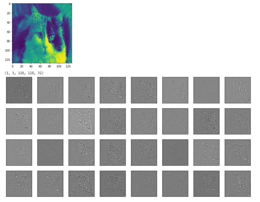
尝试在其中应用tf.image_summary函数，你应该会得到一个小图像的网格。

下面是按照这里的所有步骤所得到的图像。

- mdaoust

---

谢谢你的回答，我在转置部分卡住了。最终我使用了一个稍微不同的版本，因为我只需要看到前几个卷积（我不需要将它们全部组装成网格）。在tensorboard上检查网格有点困难。 - panmari

我觉得你最后写的fy和fx实际上应该是cy和cx。 - jeandut

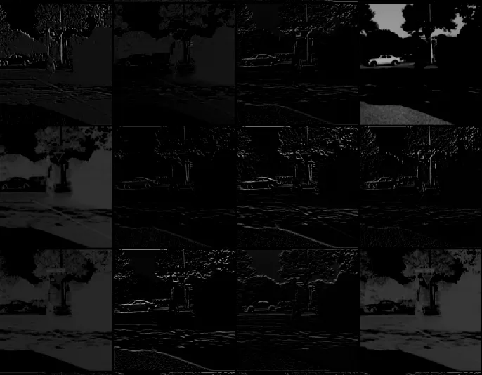
此外，您只能将4D张量传递给tf.image_summary，因此您需要重新调整形状V=tf.reshape(V,(1,4*256,8*256,1))。 - jeandut

@mdaoust 在这行代码 V = tf.image.resize_image_with_crop_or_pad(image, iy, ix) 中，第一个参数应该是 V 而不是 image 吗？我看不出来 image 是从哪里来的。 - BobbyG

我猜在这一行代码 V = tf.image.resize_image_with_crop_or_pad(image, iy, ix) 中，“image”应该被替换为“V”。对于TensorFlow的最新版本，tf.summary.image("image_name", V )也可以使用。它实际上运行得很好！ - smile

Answer 2

如果有人想要"跳转"到numpy并在那里进行可视化，这里提供一个例子来显示权重和处理结果。所有的变换都是基于mdaoust先前的回答。

# to visualize 1st conv layer Weights
vv1 = sess.run(W_conv1)

# to visualize 1st conv layer output
vv2 = sess.run(h_conv1,feed_dict = {img_ph:x, keep_prob: 1.0})
vv2 = vv2[0,:,:,:]   # in case of bunch out - slice first img


def vis_conv(v,ix,iy,ch,cy,cx, p = 0) :
    v = np.reshape(v,(iy,ix,ch))
    ix += 2
    iy += 2
    npad = ((1,1), (1,1), (0,0))
    v = np.pad(v, pad_width=npad, mode='constant', constant_values=p)
    v = np.reshape(v,(iy,ix,cy,cx)) 
    v = np.transpose(v,(2,0,3,1)) #cy,iy,cx,ix
    v = np.reshape(v,(cy*iy,cx*ix))
    return v

# W_conv1 - weights
ix = 5  # data size
iy = 5
ch = 32   
cy = 4   # grid from channels:  32 = 4x8
cx = 8
v  = vis_conv(vv1,ix,iy,ch,cy,cx)
plt.figure(figsize = (8,8))
plt.imshow(v,cmap="Greys_r",interpolation='nearest')

#  h_conv1 - processed image
ix = 30  # data size
iy = 30
v  = vis_conv(vv2,ix,iy,ch,cy,cx)
plt.figure(figsize = (8,8))
plt.imshow(v,cmap="Greys_r",interpolation='nearest')

- rgr

Answer 3

您可以尝试以下方法获取卷积层激活图像：

：

    h_conv1_features = tf.unpack(h_conv1, axis=3)
    h_conv1_imgs = tf.expand_dims(tf.concat(1, h_conv1_features_padded), -1)

这将得到一个垂直条纹，其中所有图像都被垂直连接在一起。

如果您想要它们填充（在我的relu激活情况下用白线填充）：

    h_conv1_features = tf.unpack(h_conv1, axis=3)
    h_conv1_max = tf.reduce_max(h_conv1)
    h_conv1_features_padded = map(lambda t: tf.pad(t-h_conv1_max, [[0,0],[0,1],[0,0]])+h_conv1_max, h_conv1_features)
    h_conv1_imgs = tf.expand_dims(tf.concat(1, h_conv1_features_padded), -1)

- Anton Suslov

Answer 4

我个人尝试将每个2D滤波器铺设在单个图像中。

为了做到这一点，我发现可以利用depth_to_space函数，因为它接收一个4D张量

[batch, height, width, depth]

并产生如下形状的输出：

[batch, height*block_size, width*block_size, depth/(block_size*block_size)]

其中block_size是输出图像中的“瓷砖”数量。这种方法的唯一限制是深度应该是block_size的平方，即一个整数，否则它不能正确“填充”结果图像。可能的解决方案是将输入张量的深度填充到方法接受的深度，但我还没有尝试过这种方法。

- EdoG

Answer 5

另一种我认为非常简单的方法是使用get_operation_by_name函数。我曾经尝试过其他方法来可视化层，但这个方法对我很有帮助。

#first, find out the operations, many of those are micro-operations such as add etc.
graph = tf.get_default_graph()
graph.get_operations()

#choose relevant operations
op_name = '...' 
op = graph.get_operation_by_name(op_name)
out = sess.run([op.outputs[0]], feed_dict={x: img_batch, is_training: False}) 
#img_batch is a single image whose dimensions are (1,n,n,1). 

# out is the output of the layer, do whatever you want with the output
#in my case, I wanted to see the output of a convolution layer
out2 = np.array(out)
print(out2.shape)

# determine, row, col, and fig size etc.
for each_depth in range(out2.shape[4]):
    fig.add_subplot(rows, cols, each_depth+1)
    plt.imshow(out2[0,0,:,:,each_depth], cmap='gray')

例如，以下是我的模型第二个卷积层的输入（彩色猫）和输出。 请注意，我知道这个问题很旧，并且有更简单的Keras方法，但对于使用其他人的旧模型（如我）的人来说，这可能很有用。

- smttsp