扩展至1分钟，计算平均值

Question

扩展至1分钟，计算平均值

4

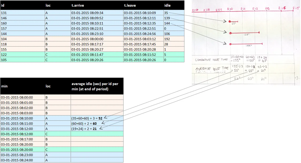
我试图通过操作时间来以每分钟为基础重新分配平均空闲时间：

#############################################################
##Reproducible example 1 (n=10):
#############################################################    df.in <- structure(list(id = c(31, 46, 60, 57, 44, 04, 18, 55, 
22, 5), loc = structure(c(1L, 1L, 1L, 1L, 1L, 2L, 2L, 2L, 
3L, 3L), .Label = c("A", "B", "C"), class = "factor"), t.arrive = structure(c(1425197374, 
1425197392, 1425197411, 1425198171, 1425198190, 1425196800, 1425197837, 
1425198027, 1425197507, 1425198026), class = c("POSIXct", "POSIXt"
), tzone = "UTC"), t.leave = structure(c(1425197409, 1425197531, 
1425197555, 1425198171, 1425198296, 1425196992, 1425197865, 1425198028, 
1425197512, 1425198026), class = c("POSIXct", "POSIXt"), tzone = "UTC"), 
    idle = c(35, 139, 144, 0, 106, 192, 28, 1, 5, 0)), .Names = c("id", 
"loc", "t.arrive", "t.leave", "idle"), class = c("tbl_df", "tbl", 
"data.frame"), row.names = c(NA, -10L))


#############################################################
##Reproducible example 2 (n=100):
#############################################################
> dput(df.in)
structure(list(id = c(78, 93, 107, 84, 104, 91, 71, 66, 189, 
182, 92, 209, 96, 84, 50, 103, 182, 183, 74, 132, 101, 78, 88, 
93, 48, 107, 82, 72, 182, 83, 66, 91, 104, 50, 71, 96, 103, 74, 
182, 101, 132, 84, 78, 88, 93, 107, 83, 182, 48, 66, 96, 51, 
75, 65, 102, 80, 106, 63, 156, 51, 75, 79, 67, 65, 85, 94, 89, 
106, 69, 80, 79, 67, 69, 52, 105, 94, 73, 95, 100, 76, 55, 99, 
60, 69, 53, 86, 52, 105, 90, 64, 95, 73, 63, 100, 76, 51, 99, 
53, 75, 52), loc = structure(c(1L, 1L, 1L, 1L, 1L, 1L, 1L, 1L, 
1L, 1L, 1L, 1L, 1L, 1L, 1L, 1L, 1L, 1L, 1L, 1L, 1L, 1L, 1L, 1L, 
1L, 1L, 1L, 1L, 1L, 1L, 1L, 1L, 1L, 1L, 1L, 1L, 1L, 1L, 1L, 1L, 
1L, 1L, 1L, 1L, 1L, 1L, 1L, 1L, 1L, 1L, 1L, 4L, 4L, 4L, 4L, 4L, 
4L, 4L, 4L, 4L, 4L, 4L, 4L, 4L, 4L, 4L, 4L, 4L, 4L, 4L, 4L, 4L, 
6L, 6L, 6L, 6L, 6L, 6L, 6L, 6L, 6L, 6L, 6L, 6L, 6L, 6L, 6L, 6L, 
6L, 6L, 6L, 6L, 6L, 6L, 6L, 6L, 6L, 6L, 6L, 6L), .Label = c("A", 
"HPB", "HPS", "B", "OPP-B", "C"), class = "factor"), t.arrive = structure(c(1425197374, 
1425197392, 1425197411, 1425197927, 1425198171, 1425198190, 1425198194, 
1425198227, 1425198303, 1425198475, 1425198812, 1425198924, 1425199119, 
1425199199, 1425199235, 1425199355, 1425199528, 1425199544, 1425199641, 
1425199643, 1425199648, 1425199801, 1425199812, 1425200087, 1425200103, 
1425200310, 1425200454, 1425200478, 1425200517, 1425200611, 1425200669, 
1425201076, 1425201105, 1425201275, 1425201287, 1425201378, 1425201536, 
1425201604, 1425201628, 1425201767, 1425201893, 1425202137, 1425202244, 
1425202255, 1425202557, 1425202566, 1425202879, 1425202962, 1425203094, 
1425203109, 1425203380, 1425196800, 1425196800, 1425197837, 1425198027, 
1425198955, 1425199074, 1425199342, 1425199465, 1425199855, 1425199929, 
1425199970, 1425200480, 1425200517, 1425200950, 1425201289, 1425201357, 
1425201879, 1425202374, 1425202982, 1425202987, 1425203318, 1425197507, 
1425198026, 1425198378, 1425198390, 1425198994, 1425199059, 1425199298, 
1425199522, 1425199528, 1425199728, 1425200115, 1425200289, 1425200373, 
1425200547, 1425200679, 1425200880, 1425200909, 1425201364, 1425201509, 
1425201801, 1425201910, 1425202039, 1425202246, 1425202490, 1425202555, 
1425202589, 1425203048, 1425203108), class = c("POSIXct", "POSIXt"
), tzone = "UTC"), t.leave = structure(c(1425197409, 1425197531, 
1425197555, 1425197927, 1425198171, 1425198296, 1425198194, 1425198315, 
1425198411, 1425198553, 1425198818, 1425198924, 1425199119, 1425199219, 
1425199235, 1425199359, 1425199528, 1425199558, 1425199652, 1425199734, 
1425199648, 1425199801, 1425200028, 1425200198, 1425200240, 1425200364, 
1425200492, 1425200619, 1425200610, 1425200910, 1425200859, 1425201100, 
1425201302, 1425201275, 1425201467, 1425201393, 1425201569, 1425201704, 
1425201805, 1425201951, 1425202057, 1425202262, 1425202370, 1425202255, 
1425202667, 1425202840, 1425202913, 1425202990, 1425203094, 1425203109, 
1425203380, 1425196992, 1425196800, 1425197865, 1425198028, 1425198984, 
1425199149, 1425199356, 1425199466, 1425199902, 1425200051, 1425200286, 
1425200783, 1425200845, 1425201125, 1425201586, 1425201640, 1425201879, 
1425202377, 1425202986, 1425202987, 1425203318, 1425197512, 1425198026, 
1425198378, 1425198486, 1425199021, 1425199078, 1425199325, 1425199558, 
1425199810, 1425199939, 1425200118, 1425200305, 1425200485, 1425200782, 
1425200894, 1425201065, 1425201111, 1425201364, 1425201623, 1425201857, 
1425202015, 1425202039, 1425202404, 1425202671, 1425202651, 1425202834, 
1425203105, 1425203198), class = c("POSIXct", "POSIXt"), tzone = "UTC"), 
    idle = c(35, 139, 144, 0, 0, 106, 0, 88, 108, 78, 6, 0, 0, 
    20, 0, 4, 0, 14, 11, 91, 0, 0, 216, 111, 137, 54, 38, 141, 
    93, 299, 190, 24, 197, 0, 180, 15, 33, 100, 177, 184, 164, 
    125, 126, 0, 110, 274, 34, 28, 0, 0, 0, 192, 0, 28, 1, 29, 
    75, 14, 1, 47, 122, 316, 303, 328, 175, 297, 283, 0, 3, 4, 
    0, 0, 5, 0, 0, 96, 27, 19, 27, 36, 282, 211, 3, 16, 112, 
    235, 215, 185, 202, 0, 114, 56, 105, 0, 158, 181, 96, 245, 
    57, 90)), class = "data.frame", .Names = c("id", "loc", "t.arrive", 
"t.leave", "idle"), row.names = c(NA, -100L))

这里是我要得到的内容：在任何给定分钟内（必须按loc分组），取每个ID贡献的闲置时间之和。然后，取平均值：

这是我尝试过的方法:

## Expand time into 1-min intervals
df.min <- df.in %>%
              rownames_to_column() %>%
              group_by(rowname) %>%  
              do(data.frame(min = seq(.$t.arrive, .$t.leave, by = "1 min"),
                            id = first(.$id),
                            loc = first(.$loc),
                            idle.mean = as.numeric(mean(.$idle))
              ))


## Round Off to 0 seconds to make it more tractable:
df.min$min <- as.POSIXct(round(df.min$min, "mins"))


## Calculate within each minute
df.min <- df.min %>% 
            group_by(min, loc) %>% 
            summarise(units.count = n(),
                      cum.queue.min = sum(idle.mean)/60
                      )

## Take 1 min average idle time per id
df.min <- as.data.frame(df.min)
df.min <- df.min %>%
            mutate(queue.tmean = cum.queue.min / units.count) %>%
            select(-units.count, -cum.queue.min) %>%
            arrange(min, loc)

- Thomas Speidel

我不确定您是否希望解决方案“在任何给定的分钟内（必须按位置分组），取每个ID贡献的空闲时间总和。然后，取平均值”，这是我的解决方案，还是根据您提供的图像进行解决，我相信其他解决方案可以做到。虽然它们得出的结果不同。 - David Rubinger

我想要在任何给定的分钟内（按位置分组）得到平均值。显然，平均值需要求和。在图表中，我试图说明逻辑和构建块，但它包括任何给定分钟的平均空闲时间。唯一未说明的步骤是四舍五入到最接近的分钟。我这样做是为了简化问题。 - Thomas Speidel

谢谢。为了更具体，您在第8分09秒时期望loc=A的结果是什么？ - David Rubinger

如果我要将t.arrive四舍五入到最接近的一分钟（这是我选择的方法），那么8:09就不应该存在，如果确实存在，平均空闲时间应该为“NA”（而不是零）。 - Thomas Speidel

3个回答

2

data.table方法

data.table方法非常高效，无需循环。

library(lubridate)
library(data.table)
setDT(dt.in)
dt.in[, arrive_min := round_date(t.arrive, "mins")]
dt2 <- dt.in[, .(mins = arrive_min + (0:floor(idle/60))*60) , by = .(id, loc, arrive_min)]

这个总结假设每个分组变量都有唯一的arrive_min，通过将arrive_min添加到分组变量中自动满足这个条件。（参见下面不规则的示例。早期的解决方案由于arrive_min不唯一而抛出differing rows错误）。一旦我们解决了这些问题，剩下的就很简单了。

dt.in[, mins:=arrive_min, ]
dt_full <- dt.in[dt2, on = c("id", "loc", "mins")]
dt_full[, .(mins = mins, idle=c(rep(60, idle[1]/60), idle[1]%%60)), by = .(id, loc, i.arrive_min)
   ][, .(ave_idle=mean(idle)), by = .(mins, loc)]


#                   min1 loc ave_idle
# 1: 2015-03-01 08:10:00   A 51.66667
# 2: 2015-03-01 08:11:00   A 60.00000
# 3: 2015-03-01 08:12:00   A 21.50000
# 4: 2015-03-01 08:23:00   A 30.00000
# 5: 2015-03-01 08:24:00   A 46.00000
# 6: 2015-03-01 08:00:00   B 60.00000
# 7: 2015-03-01 08:01:00   B 60.00000
# 8: 2015-03-01 08:02:00   B 60.00000
# 9: 2015-03-01 08:03:00   B 12.00000
#10: 2015-03-01 08:17:00   B 28.00000
#11: 2015-03-01 08:20:00   B  1.00000
#12: 2015-03-01 08:12:00   C  5.00000
#13: 2015-03-01 08:20:00   C  0.00000

请注意，在创建mins = arrive_min + (0:floor(idle/60))*60和idle=c( rep(60, idle[1]/60), idle[1]%%60)时，我们假设对于每个分组变量（id、loc、arrive_min），存在唯一的idle。前者将t.arrive=08:01:00，idle=159转换为mins=c(08:01:00, 08:02:00, 08:03:00)，后者将c(159, NA , NA)转换为c(60, 60, 39)。因此，如果您有如下数据点，则应修改此方法：

  id loc            t.arrive             t.leave    idle
1 78   A 2015-03-01 08:09:36 2015-03-01 08:09:58      22
2 78   A 2015-03-01 08:09:34 2015-03-01 08:10:09      35

dplyr

我们可以使用 dplyr。与 data.table 相比，do 操作有些笨拙。

df.in <- df.in %>% 
  mutate(arrive_min=round_date(t.arrive, "mins"))
df2 <- df.in %>% 
  group_by(id, loc, arrive_min) %>% 
  do(data.frame(id=.$id, loc=.$loc, mins = .$arrive_min + (0:floor(.$idle/60))*60))
df.in$mins <- df.in$arrive_min
left_join(df2, df.in, by=c("id", "loc", "mins")) %>%  
  group_by(id, loc, arrive_min.x) %>% 
  do(data.frame(min1=.$mins, idle=c(rep(60, .$idle[1]/60), .$idle[1]%%60))) %>% 
  group_by(min1, loc) %>% 
  summarise(ave_idle=mean(idle)) 


#                  min1  loc.x ave_idle
#                <dttm> <fctr>    <dbl>
#1  2015-03-01 08:00:00      B 60.00000
#2  2015-03-01 08:01:00      B 60.00000
#3  2015-03-01 08:02:00      B 60.00000
#4  2015-03-01 08:03:00      B 12.00000
#5  2015-03-01 08:10:00      A 51.66667
#6  2015-03-01 08:11:00      A 60.00000
#7  2015-03-01 08:12:00      A 21.50000
#8  2015-03-01 08:12:00      C  5.00000
#9  2015-03-01 08:17:00      B 28.00000
#10 2015-03-01 08:20:00      B  1.00000
#11 2015-03-01 08:20:00      C  0.00000
#12 2015-03-01 08:23:00      A 30.00000
#13 2015-03-01 08:24:00      A 46.00000

- ExperimenteR

谢谢！我想利用data.table的效率（虽然我没有经验），因为我的数据很大。这在完整数据上会产生许多错误。dt2 <- df.in[, .(min1 = min1 + (0:floor(idle/60))*60) , by = .(id, loc)]会出现以下警告信息：警告信息： 1：在0:floor(idle/60)中：数值表达式有1608个元素：只使用了第一个和12：在unclass(e1) + unclass(e2)中：较长的对象长度不是较短的对象长度的倍数。 - Thomas Speidel

类似的错误：`+ do(data.frame(id=.$id, loc=.$loc, min1 = .$min1 + (0:floor(.$idle/60))*60)) Error in data.frame(id = .$id, loc = .$loc, min1 = .$min1 + (0:floor(.$idle/60)) * : 参数暗示了不同数量的行：9，11 此外：有50个或更多警告（使用warnings()查看前50个）

warnings() 警告信息： 1：在0:floor(.$idle/60)中：数值表达式有1507个元素：仅使用第一个 2：在unclass(e1) + unclass(e2)中：较长的对象长度不是较短对象长度的倍数`

- Thomas Speidel

1

你能提供一个可以重现错误的数据集实例吗？ - ExperimenteR

@ThomasSpeidel 我已经更新了解决方案。希望错误的源头现在更加透明。 - ExperimenteR

1

我认为这就是你要找的内容：

# Create sequence of datetimes by second from t.arrive to t.leave for each observation
df <- NULL
for (i in 1:nrow(df.in)) {
    df <- bind_rows(
        df,
        slice(data_frame(  # slice cuts off last second entry
            t.present = seq(df.in[[i, 't.arrive']], df.in[[i, 't.leave']], by = 'sec'),
            id = df.in[[i, 'id']],
            loc = df.in[[i, 'loc']]), -n()))
}

# Calculate target metric
df$t.present.min <- as.POSIXct(trunc(df$t.present, 'mins'))
result <- df %>%
    group_by(id, loc, t.present.min) %>%
    summarise(secs.present = n()) %>%
    group_by(loc, t.present.min) %>%
    summarise(avg.secs = mean(secs.present))
result

结果：

      loc       t.present.min avg.secs
   <fctr>              <dttm>    <dbl>
1       A 2015-03-01 08:09:00 17.00000
2       A 2015-03-01 08:10:00 39.33333
3       A 2015-03-01 08:11:00 60.00000
4       A 2015-03-01 08:12:00 23.00000
5       A 2015-03-01 08:23:00 50.00000
6       A 2015-03-01 08:24:00 56.00000
7       B 2015-03-01 08:00:00 60.00000
8       B 2015-03-01 08:01:00 60.00000
9       B 2015-03-01 08:02:00 60.00000
10      B 2015-03-01 08:03:00 12.00000
11      B 2015-03-01 08:17:00 28.00000
12      B 2015-03-01 08:20:00  1.00000
13      C 2015-03-01 08:11:00  5.00000

- David Rubinger

网页内容由stack overflow 提供, 点击上面的

可以查看英文原文，
原文链接

- Weihuang Wong · Accepted Answer

一种方法是创建一个数据框，其中每行都由id-loc-time标识，其中每个时间为一分钟，值为该时间的空闲秒数，例如：

  id loc                time secs
1 46   A 2015-03-01 08:10:00   60
2 46   A 2015-03-01 08:11:00   60
3 46   A 2015-03-01 08:12:00   19

一个简单的函数，可以根据起始时间、空闲秒数和其他标识符创建这样的数据框：

library(lubridate)
make_obs <- function(start, idle, id, loc) {
  st <- round_date(start, "min")
  mins <- trunc(idle / 60)
  times <- c(st, if (mins > 0) st + minutes(1 : mins))
  data.frame(
    id = id, loc = loc, time = times, secs = c(rep(60, mins), idle %% 60)
    )
}

然后使用mapply来遍历原始数据集，并使用dplyr函数进行聚合：

library(dplyr)
out <- do.call(rbind, mapply(make_obs, 
  df.in$t.arrive, df.in$idle, df.in$id, df.in$loc,
  SIMPLIFY = FALSE))
group_by(out, loc, time) %>%
  summarise(idle = mean(secs))

输出：

Source: local data frame [13 x 3]
Groups: loc [?]

      loc                time     idle
   <fctr>              <dttm>    <dbl>
1       A 2015-03-01 08:10:00 51.66667
2       A 2015-03-01 08:11:00 60.00000
3       A 2015-03-01 08:12:00 21.50000
4       A 2015-03-01 08:23:00 30.00000
...