我有一个周期为T的函数,想知道如何获取傅里叶系数列表。我尝试使用numpy中的fft模块,但它似乎更专注于傅里叶变换而不是级数。
也许这是缺乏数学知识的原因,但我无法从fft中计算傅里叶系数。
感谢提供帮助和/或示例。
5个回答
36
最后,最简单的方法(使用黎曼和计算系数)是解决我的问题最便携/高效/稳健的方式:
给我: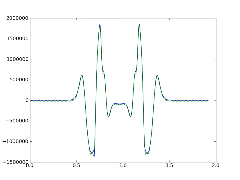
import numpy as np
def cn(n):
   c = y*np.exp(-1j*2*n*np.pi*time/period)
   return c.sum()/c.size

def f(x, Nh):
   f = np.array([2*cn(i)*np.exp(1j*2*i*np.pi*x/period) for i in range(1,Nh+1)])
   return f.sum()

y2 = np.array([f(t,50).real for t in time])

plot(time, y)
plot(time, y2)
给我:
- Mermoz
5
谢谢您发布这个解决方案,它帮我节省了一些时间 :) - zega
谢谢。正是我想要的。 - Thoth19
6可以提供一个有注释的最小工作示例吗? - SeSodesa
@SeSodesa,请参考此问题中的工作示例:https://dev59.com/a7Hma4cB1Zd3GeqPQsUS。请注意,数据并不是周期性的。此外,请参考此处的答案https://dev59.com/a7Hma4cB1Zd3GeqPQsUS#54639960,以了解缩放和计算c[0]的方法。 - makeyourownmaker
既然最终你只是绘制
y2 的实部,为什么不直接使用 np.cos(...) 计算它,而不是使用 np.exp(1j...)? - Tropilio21
这是一个旧问题,但由于我必须编写代码,所以在此发布使用
以下是实现方式,它允许通过传递适当的
这是一个使用示例:
numpy.fft 模块的解决方案,该模块可能比其他手工制作的解决方案更快。
DFT 是计算函数的傅里叶级数系数的正确工具,该函数定义为参数的分析表达式或某些离散点上的数值插值函数,可精确计算。以下是实现方式,它允许通过传递适当的
return_complex 来计算傅里叶级数的实值系数或复值系数:def fourier_series_coeff_numpy(f, T, N, return_complex=False):
"""Calculates the first 2*N+1 Fourier series coeff. of a periodic function.
Given a periodic, function f(t) with period T, this function returns the
coefficients a0, {a1,a2,...},{b1,b2,...} such that:
f(t) ~= a0/2+ sum_{k=1}^{N} ( a_k*cos(2*pi*k*t/T) + b_k*sin(2*pi*k*t/T) )
If return_complex is set to True, it returns instead the coefficients
{c0,c1,c2,...}
such that:
f(t) ~= sum_{k=-N}^{N} c_k * exp(i*2*pi*k*t/T)
where we define c_{-n} = complex_conjugate(c_{n})
Refer to wikipedia for the relation between the real-valued and complex
valued coeffs at http://en.wikipedia.org/wiki/Fourier_series.
Parameters
----------
f : the periodic function, a callable like f(t)
T : the period of the function f, so that f(0)==f(T)
N_max : the function will return the first N_max + 1 Fourier coeff.
Returns
-------
if return_complex == False, the function returns:
a0 : float
a,b : numpy float arrays describing respectively the cosine and sine coeff.
if return_complex == True, the function returns:
c : numpy 1-dimensional complex-valued array of size N+1
"""
# From Shanon theoreom we must use a sampling freq. larger than the maximum
# frequency you want to catch in the signal.
f_sample = 2 * N
# we also need to use an integer sampling frequency, or the
# points will not be equispaced between 0 and 1. We then add +2 to f_sample
t, dt = np.linspace(0, T, f_sample + 2, endpoint=False, retstep=True)
y = np.fft.rfft(f(t)) / t.size
if return_complex:
return y
else:
y *= 2
return y[0].real, y[1:-1].real, -y[1:-1].imag
这是一个使用示例:
from numpy import ones_like, cos, pi, sin, allclose
T = 1.5  # any real number

def f(t):
    """example of periodic function in [0,T]"""
    n1, n2, n3 = 1., 4., 7.  # in Hz, or nondimensional for the matter.
    a0, a1, b4, a7 = 4., 2., -1., -3
    return a0 / 2 * ones_like(t) + a1 * cos(2 * pi * n1 * t / T) + b4 * sin(
        2 * pi * n2 * t / T) + a7 * cos(2 * pi * n3 * t / T)


N_chosen = 10
a0, a, b = fourier_series_coeff_numpy(f, T, N_chosen)

# we have as expected that
assert allclose(a0, 4)
assert allclose(a, [2, 0, 0, 0, 0, 0, -3, 0, 0, 0])
assert allclose(b, [0, 0, 0, -1, 0, 0, 0, 0, 0, 0])
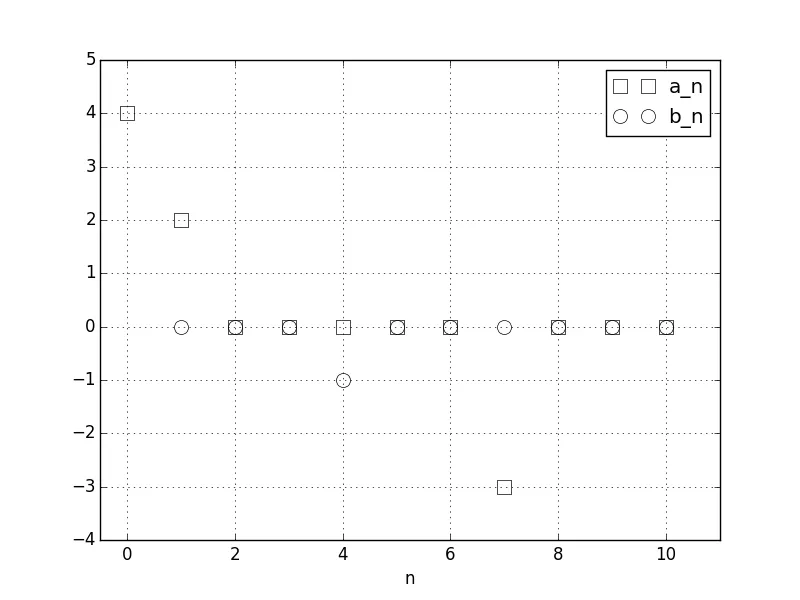
并且由此产生的系数 a0,a1,...,a10,b1,b2,...,b10 的图示如下:
这是函数的可选测试,适用于两种操作模式。在运行代码之后,您应该运行此测试,或者定义一个周期函数 f 和一个周期 T。
# #### test that it works with real coefficients:
from numpy import linspace, allclose, cos, sin, ones_like, exp, pi, \
    complex64, zeros


def series_real_coeff(a0, a, b, t, T):
    """calculates the Fourier series with period T at times t,
       from the real coeff. a0,a,b"""
    tmp = ones_like(t) * a0 / 2.
    for k, (ak, bk) in enumerate(zip(a, b)):
        tmp += ak * cos(2 * pi * (k + 1) * t / T) + bk * sin(
            2 * pi * (k + 1) * t / T)
    return tmp


t = linspace(0, T, 100)
f_values = f(t)
a0, a, b = fourier_series_coeff_numpy(f, T, 52)
# construct the series:
f_series_values = series_real_coeff(a0, a, b, t, T)
# check that the series and the original function match to numerical precision:
assert allclose(f_series_values, f_values, atol=1e-6)

# #### test similarly that it works with complex coefficients:

def series_complex_coeff(c, t, T):
    """calculates the Fourier series with period T at times t,
       from the complex coeff. c"""
    tmp = zeros((t.size), dtype=complex64)
    for k, ck in enumerate(c):
        # sum from 0 to +N
        tmp += ck * exp(2j * pi * k * t / T)
        # sum from -N to -1
        if k != 0:
            tmp += ck.conjugate() * exp(-2j * pi * k * t / T)
    return tmp.real

f_values = f(t)
c = fourier_series_coeff_numpy(f, T, 7, return_complex=True)
f_series_values = series_complex_coeff(c, t, T)
assert allclose(f_series_values, f_values, atol=1e-6)
- gg349
1
11
由于数据必须被离散采样,因此Numpy并不是计算傅里叶级数分量的正确工具。你真正想要使用像Mathematica这样的工具或者应该使用傅里叶变换。
为了粗略地进行计算,我们可以考虑一些简单的东西,比如周期为2pi的三角波,我们可以轻松地计算出傅里叶系数(c_n = -i ((-1)^(n+1))/n,其中n > 0;例如,当n=1、2、3、4、5、6时,c_n = { -i, i/2, -i/3, i/4, -i/5, i/6, ... }(使用Sum( c_n exp(i 2 pi n x) )作为傅里叶级数)。
import numpy
x = numpy.arange(0,2*numpy.pi, numpy.pi/1000)
y = (x+numpy.pi/2) % numpy.pi - numpy.pi/2
fourier_trans = numpy.fft.rfft(y)/1000
如果您查看前几个傅里叶分量:
array([ -3.14159265e-03 +0.00000000e+00j,
         2.54994550e-16 -1.49956612e-16j,
         3.14159265e-03 -9.99996710e-01j,
         1.28143395e-16 +2.05163971e-16j,
        -3.14159265e-03 +4.99993420e-01j,
         5.28320925e-17 -2.74568926e-17j,
         3.14159265e-03 -3.33323464e-01j,
         7.73558750e-17 -3.41761974e-16j,
        -3.14159265e-03 +2.49986840e-01j,
         1.73758496e-16 +1.55882418e-17j,
         3.14159265e-03 -1.99983550e-01j,
        -1.74044469e-16 -1.22437710e-17j,
        -3.14159265e-03 +1.66646927e-01j,
        -1.02291982e-16 -2.05092972e-16j,
         3.14159265e-03 -1.42834113e-01j,
         1.96729377e-17 +5.35550532e-17j,
        -3.14159265e-03 +1.24973680e-01j,
        -7.50516717e-17 +3.33475329e-17j,
         3.14159265e-03 -1.11081501e-01j,
        -1.27900121e-16 -3.32193126e-17j,
        -3.14159265e-03 +9.99670992e-02j,
首先忽略由于浮点精度导致接近0的分量(~1e-16,视为零)。更难的部分是要看到在将其除以1000的周期之前产生的3.14159数值也应该被认为是零,因为函数是周期性的。因此,如果我们忽略这两个因素,我们得到:
fourier_trans = [0,0,-i,0,i/2,0,-i/3,0,i/4,0,-i/5,0,-i/6, ...
你可以看到傅里叶级数的数字每隔一个数字出现一次(我没有进行调查,但我相信这些组件对应[c0、c-1、c1、c-2、c2,...])。我使用的约定是根据维基百科: http://en.wikipedia.org/wiki/Fourier_series。
同样,我建议使用Mathematica或能够积分和处理连续函数的计算机代数系统。
- dr jimbob
1
1理解结果需要付出一些努力,这是一个非常好的观点。+1。 - mtrw
4
您是否有函数的离散样本列表,或者函数本身是离散的?如果是这样,使用FFT算法计算的离散傅里叶变换可以直接提供傅里叶系数(请参见此处)。
另一方面,如果您拥有函数的解析表达式,则可能需要某种符号数学求解器。
- mtrw
网页内容由stack overflow 提供, 点击上面的可以查看英文原文,
原文链接
原文链接
sympy解决Krezig高级工程数学中一些问题的示例! - Pradeep Padmanaban C