在sklearn的逻辑回归中，C参数是什么意思？

Question

在`sklearn.linear_model.LogisticRegression`中，C参数的含义是什么？它如何影响决策边界？高值的C是否会使决策边界变得非线性？如果我们可视化决策边界，逻辑回归的过拟合会呈现怎样的特征？

- Abdulwahab Almestekawy

---

这回答了你的问题吗？[逻辑回归中正则化强度的倒数是什么？它应该如何影响我的代码？] (https://dev59.com/c2Ah5IYBdhLWcg3wE_1P) - padaleiana

它只回答了问题的第一部分（C参数的含义是什么）。我关心的是可视化部分（即它如何影响决策边界的形状）。我希望有人能提供一个带有可视化示例的例子。 - Abdulwahab Almestekawy

我可以想象非线性决策边界（蜿蜒的线）的过拟合情况，但对于像逻辑回归这样的线性模型，我们如何使用不同的C值来想象决策边界的形状呢？ - Abdulwahab Almestekawy

Answer 1

来自文档：

C: 浮点数，默认值为1.0。 正则化强度的倒数；必须是一个正浮点数。与支持向量机类似，较小的值指定了更强的正则化。

如果你不理解这个，可以在Cross Validated上询问比在这里好。

尽管计算机科学人员经常把函数的所有参数都称为“参数”，但在机器学习中，C被称为“超参数”。参数是告诉模型如何处理特征的数字，而超参数告诉模型如何选择参数。

正则化通常指更极端的参数应该有复杂度惩罚的概念。这个想法是，只看训练数据而不关注参数的极端程度会导致过度拟合。C的高值告诉模型要给予训练数据更高的权重，而对复杂度惩罚给予较低的权重。低值告诉模型要更多地考虑复杂度惩罚，以代价适配训练数据。基本上，高C意味着“非常相信这些训练数据”，而低值表示“这些数据可能不能完全代表真实世界数据，所以如果它让你使参数非常大，就不要听它的”。

https://zh.wikipedia.org/wiki/正则化

- Acccumulation

---

请您能否提供一个低C值和高C值之间决策边界差异的例子？据我所知，逻辑回归始终具有线性决策边界，那么它如何在大C值下拥有灵活的决策边界呢？ - Abdulwahab Almestekawy

Answer 2

什么是正则化？

逻辑回归是一个最小化代价函数的优化问题。正则化在这个代价函数中添加了一个惩罚项，从本质上改变了目标函数，使得问题与没有惩罚项时不同。惩罚项由模型的系数组成，通过添加惩罚项来惩罚大的系数（因为大的系数会增加被最小化的目标函数的值），并且“人为地”使它们变小。

如果模型过拟合（一个经典的例子是它有太多的变量），正则化可以帮助。如果没有过拟合，则不需要正则化。下面的图表将展示两者之间的区别。

通过对数似然函数进行内部优化的一种简单方法是使用以下两行代码。

scores = X.dot(coefficients) + intercept
log_likelihood = np.sum((y-1)*scores - np.log(1 + np.exp(-scores)))

正则化会添加一个惩罚项，因此现在对数似然函数看起来是这样的：

penalty_term = (1 / C if C else 0) * np.sum(coefficients**2)   # only regularize non-intercept coefficients
log_likelihood = np.sum((y-1)*scores - np.log(1 + np.exp(-scores))) - penalty_term
#                                                                   ^^^^^^^^^^^^^^  <--- penalty here

如果我们要从头开始编写一个逻辑回归模型，它将只是一个循环，在每一步中，系数会被更新以使误差变得越来越小。

from sklearn.datasets import make_classification
import numpy as np

def logistic_regression(X, y, C=None, step_size=0.005):
    
    coef_ = np.array([0.]*X.shape[1])
    l2_penalty = 1 / C if C else 0
    
    for ctr in range(100):
        # predict P(y_i = 1 | X_i, coef_)
        predicted_proba = 1 / (1 + np.exp(-X.dot(coef_)))
        errors = y - predicted_proba
        # add penalty only for non-intercept 
        penalty = 2*l2_penalty*coef_*[0, *[1]*(len(coef_)-1)]
        # compute derivatives and add penalty
        derivatives = X.T.dot(errors) - penalty
        # update the coefficients
        coef_ += step_size * derivatives
        
    return coef_

def log_likelihood(X, y, coef_, C=None):
    penalty_term = (1 / C if C else 0) * np.sum(coef_[1:]**2)
    scores = X.dot(coef_)
    return np.sum((y-1)*scores - np.log(1 + np.exp(-scores))) - penalty_term

def compute_accuracy(X, y, coef_):
    predictions = (X.dot(coef_) > 0)
    return np.mean(predictions == y)


# example
X, y = make_classification()
X_ = np.c_[[1]*100, X]
coefs = logistic_regression(X_, y, C=0.01)
accuracy = compute_accuracy(X_, y, coefs)

scikit-learn的LogisticRegression默认进行正则化(?!)

如果我们回顾一下之前提到的scikit-learn，由于正则化会使系数变小，所以将数据输入模型时很重要要对其进行缩放（可以使用StandardScaler()）。因为系数的大小取决于变量的尺度。然而，令人费解的是，scikit-learn的LogisticRegression默认进行正则化��如文档中所述，默认值为C: float, default=1.0），你实际上需要设置penalty=None来求解非正则化的系数。

不过拟合与未拟合模型的决策边界

如之前提到的，如果模型没有过拟合，就不需要进行正则化（所以在scikit-learn中应该设置penalty=None）。下面的图显示了两个训练模型的类别区域（使用等高线图表示），一个是没有进行正则化的模型，另一个是进行了正则化的模型。没有进行正则化的模型在测试数据上表现更好，这也得到了通过绘制的类别区域的确认。

现在，如果模型过拟合（没有正则化的类别区域看起来非常荒谬，并且适应了大量训练数据中的噪声），那么正则化是有用的，这一点通过带有正则化的模型的测试准确性得到了确认。

---

用于生成等高线图的代码。

import numpy as np
import matplotlib.pyplot as plt
from sklearn.datasets import make_circles
from sklearn.model_selection import train_test_split
from sklearn.preprocessing import PolynomialFeatures
from sklearn.linear_model import LogisticRegression
from matplotlib.colors import ListedColormap

def plot_class_regions(clf, transformer, X, y, ax=None):

    if ax is None:
        fig, ax = plt.subplots(figsize=(6,6))
    
    # lighter cmap for contour filling and darker cmap for markers
    cmap_light = ListedColormap(['lightgray', 'khaki'])
    cmap_bold  = ListedColormap(['black', 'yellow'])

    # create a sample for contour plot
    x_min, x_max = X[:, 0].min()-0.5, X[:, 0].max()+0.5
    y_min, y_max = X[:, 1].min()-0.5, X[:, 1].max()+0.5
    x2, y2 = np.meshgrid(np.arange(x_min, x_max, 0.03), np.arange(y_min, y_max, 0.03))
    
    # transform sample
    sample = np.c_[x2.ravel(), y2.ravel()]
    if transformer:
        sample = transformer.transform(sample)
        
    # make predictions
    preds = clf.predict(sample).reshape(x2.shape)
    # plot contour
    ax.contourf(x2, y2, preds, cmap=cmap_light, alpha=0.8)
    # scatter plot
    ax.scatter(X[:, 0], X[:, 1], c=y, cmap=cmap_bold, s=50, edgecolor='black', label='Train')
    ax.set(xlim=(x_min, x_max), ylim=(y_min, y_max))
    
    return ax

def plotter(X, y):
    
    # train-test-split
    X_train, X_test, y_train, y_test = train_test_split(X, y, random_state=0)
    # add more features
    poly = PolynomialFeatures(degree=6)
    X_poly = poly.fit_transform(X_train)

    fig, axs = plt.subplots(1, 2, figsize=(12,4), facecolor='white')

    for i, lr in enumerate([LogisticRegression(penalty=None, max_iter=10000), 
                            LogisticRegression(max_iter=2000)]):
        
        lr.fit(X_poly, y_train)

        plot_class_regions(lr, poly, X_train, y_train, axs[i])
        axs[i].scatter(X_test[:, 0], X_test[:, 1], c=y_test, cmap=ListedColormap(['black', 'yellow']), 
                   s=50, marker='^', edgecolor='black', label='Test')
        axs[i].set_title(f"{'No' if i == 0 else 'With'} penalty\nTest accuracy = {lr.score(poly.transform(X_test), y_test)}")
        axs[i].legend()
        
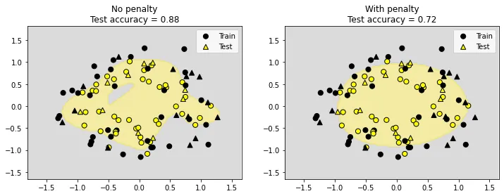
# not overfit -- no need for regularization
X, y = make_circles(factor=0.7, noise=0.2, random_state=2023)
plotter(X, y)

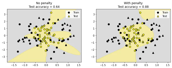
# overfit -- needs regularization
X, y = make_circles(factor=0.3, noise=0.2, random_state=2023)
X[:, 1] += np.random.default_rng(2023).normal(size=len(X))
plotter(X, y)

- cottontail