raster::rasterToContour；轮廓线不连续

Question

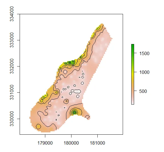
我正在尝试使用R中的raster包从栅格对象中提取等高线。 rasterToContour似乎工作得很好，并且绘制得很漂亮，但是当进行调查时，发现等高线被分成了不规则的段。来自?rasterToContour的示例数据。

library(raster)

f <- system.file("external/test.grd", package="raster")
r <- raster(f)
x <- rasterToContour(r)
class(x)
plot(r)
plot(x, add=TRUE)

我正在尝试从栅格中提取样本站点的轮廓线。因此，我们选择一个随机站点，提取其高程，并再次运行rasterToContour()，指定轮廓线level的高程。

# our sample site - a random cell chosen on the raster
xyFromCell(r, 5000) %>%
  SpatialPoints(proj4string = crs(r)) %>%
  {. ->> site_sp} %>%
  st_as_sf %>%
  {. ->> site_sf}

# find elevation of sample site, and extract contour lines
extract(r, site_sf) %>%
  {. ->> site_elevation}

# extract contour lines
r %>%
  rasterToContour(levels = site_elevation) %>%
  {. ->> contours_sp} %>%
  st_as_sf %>%
  {. ->> contours_sf}

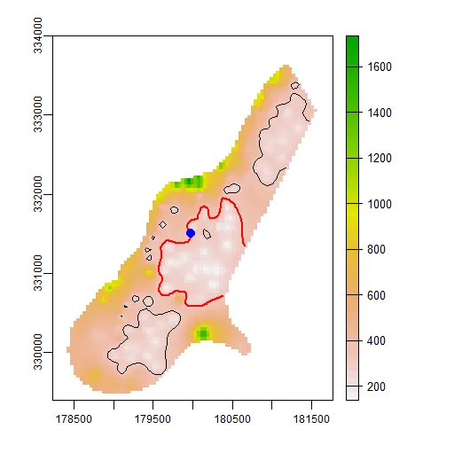
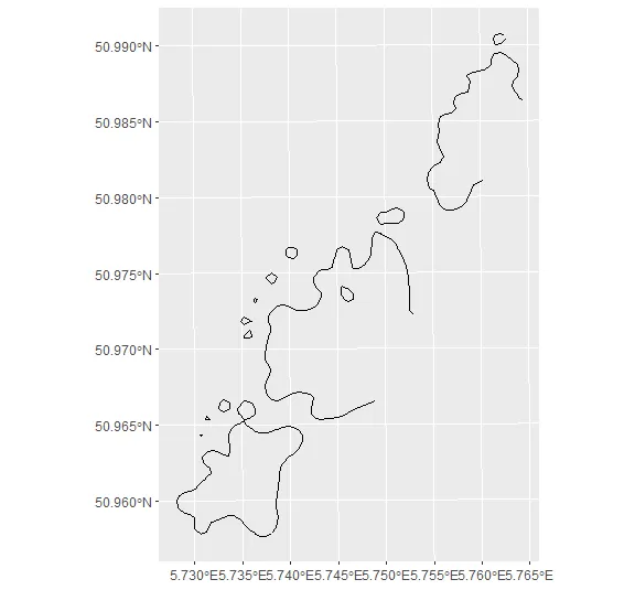
# plot the site and new contour lines (approx elevation 326)
plot(r)
plot(contours_sf, add = TRUE)
plot(site_sf, add = TRUE)

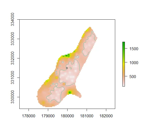
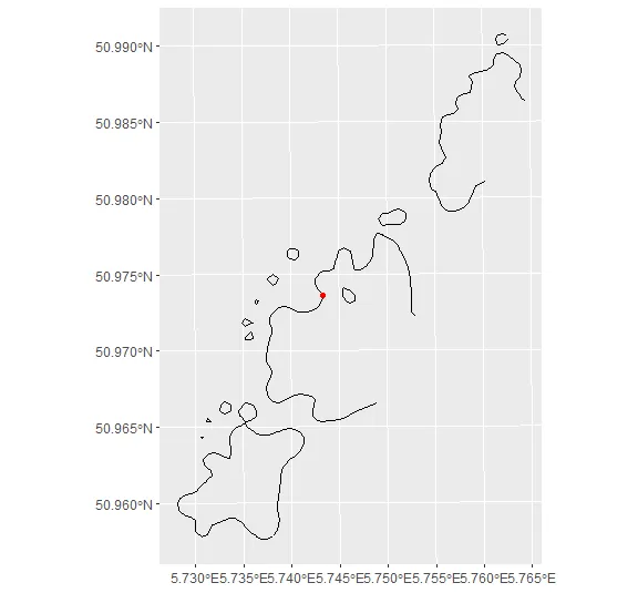
# plot the contour lines and sample site - using sf and ggplot
ggplot()+
  geom_sf(data = contours_sf)+
  geom_sf(data = site_sf, color = 'red')

然后我们使用st_intersects函数来查找与站点相交的线（缓冲宽度为100以确保它与线接触）。但是，这会返回所有等高线。

contours_sf %>%
  filter(
    st_intersects(., site_sf %>% st_buffer(100), sparse = FALSE)[1,]
  ) %>%
  ggplot()+
  geom_sf()

我认为所有的行都被返回了，因为它们似乎是一个单独的MULTILINESTRINGsf对象。

contours_sf

# Simple feature collection with 1 feature and 1 field
# geometry type:  MULTILINESTRING
# dimension:      XY
# bbox:           xmin: 178923.1 ymin: 329720 xmax: 181460 ymax: 333412.3
# CRS:            +proj=sterea +lat_0=52.1561605555556 +lon_0=5.38763888888889 +k=0.9999079 +x_0=155000 +y_0=463000 +datum=WGS84 +units=m +no_defs
# level                       geometry
# C_1 326.849822998047 MULTILINESTRING ((179619.3 ...

所以，我已经使用ngeo::st_segments()将contours_sfMULTILINESTRING拆分成单独的线条（我找不到任何sf方法来做到这一点，但如果这是问题，我可以使用替代方法，特别是如果这是问题）。出乎意料的是，这返回了394个要素；从图中看，我预计大约有15条分离的线条。

contours_sf %>%
  nngeo::st_segments()

# Simple feature collection with 394 features and 1 field
# geometry type:  LINESTRING
# dimension:      XY
# bbox:           xmin: 178923.1 ymin: 329720 xmax: 181460 ymax: 333412.3
# CRS:            +proj=sterea +lat_0=52.1561605555556 +lon_0=5.38763888888889 +k=0.9999079 +x_0=155000 +y_0=463000 +datum=WGS84 +units=m +no_defs
# First 10 features:
#   level                         result
# 1  326.849822998047 LINESTRING (179619.3 329739...
# 2  326.849822998047 LINESTRING (179580 329720.4...
# 3  326.849822998047 LINESTRING (179540 329720, ...
# 4  326.849822998047 LINESTRING (179500 329735.8...
# 5  326.849822998047 LINESTRING (179495.3 329740...
# 6  326.849822998047 LINESTRING (179460 329764, ...
# 7  326.849822998047 LINESTRING (179442.6 329780...
# 8  326.849822998047 LINESTRING (179420 329810, ...
# 9  326.849822998047 LINESTRING (179410.2 329820...
# 10 326.849822998047 LINESTRING (179380 329847.3...

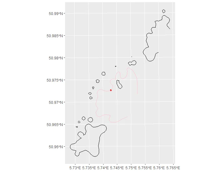
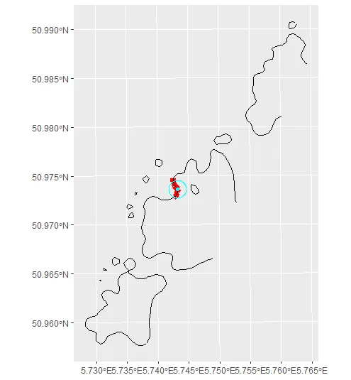
然后，当我们过滤以保留与站点相交的线（缓冲区宽度为100）时，只返回了预期等高线的一小部分（红色线段，我认为反映了100缓冲区宽度）。

contours_sf %>%
  nngeo::st_segments() %>%
  filter(
    # this syntax used as recommended by this answer https://dev59.com/vLXna4cB1Zd3GeqPEhEJ#57025700
    st_intersects(., site_sf %>% st_buffer(100), sparse = FALSE)
  ) %>%

  ggplot()+
  geom_sf(colour = 'red', size = 3)+
  geom_sf(data = contours_sf)+
  geom_sf(data = site_sf, colour = 'cyan')+
  geom_sf(data = site_sf %>% st_buffer(100), colour = 'cyan', fill = NA)

有人对以下几点有想法吗：

1. 解释为什么等高线是“断裂的”
2. 提供一种有效的方法来“连接”这些断裂的部分
3. 如果 nngeo::st_segments() 确实是 394 条线而不是 ~15 条线的来源，那么可以考虑另一种方法

- hugh-allan

Answer 1

将 MULTILINESTRING 转换为 LINESTRING 似乎可以满足您的需求：

contours_sf %>% st_cast("LINESTRING") %>% 
  filter(st_intersects(., st_buffer(site_sf, 100), sparse=FALSE)[,1]) %>%

ggplot()+
  geom_sf(data = contours_sf)+
  geom_sf(data = site_sf, color = 'red') +
  geom_sf(color = 'pink') 

- Miff

Answer 2

如果您从分解行开始进行可能会更有效

library(raster)
f <- system.file("external/test.grd", package="raster")
r <- raster(f)
x <- rasterToContour(r)
x <- disaggregate(x)

或使用 terra

library(terra)
r <- rast(f)
x <- as.contour(r)

x
# class       : SpatVector 
# geometry    : lines 
# dimensions  : 8, 1  (geometries, attributes)

x <- disaggregate(x)
x
# class       : SpatVector 
# geometry    : lines 
# dimensions  : 56, 1  (geometries, attributes)

你可以继续像这样进行

y <- st_as_sf(x)

或者像这样

r <- rast(system.file("ex/meuse.tif", package="terra"))
site <- vect(xyFromCell(r, 5000), crs=crs(r))
elevation <- extract(r, site)
v <- disaggregate(as.contour(r, levels=elevation))
i <- which.min(distance(site, v))
vv <- v[i]

plot(r)
lines(v)
lines(vv, col="red", lwd=2)
points(site, col="blue", cex=2)

- Robert Hijmans

---

谢谢@Robert，这两个选项都很好用。 - hugh-allan