我使用有限元方法来逼近Laplace方程 ,将其转换为矩阵系统AU=F,其中A是刚度向量,解出U(对我的问题不是非常重要)。现在我已经得到了近似的U,在计算AU时应该得到类似F的向量,其中F为:
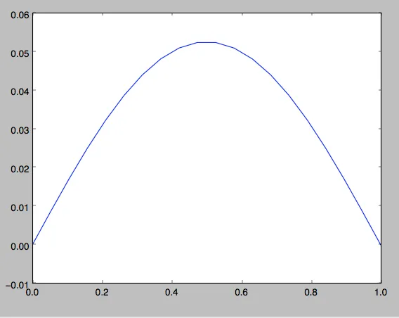
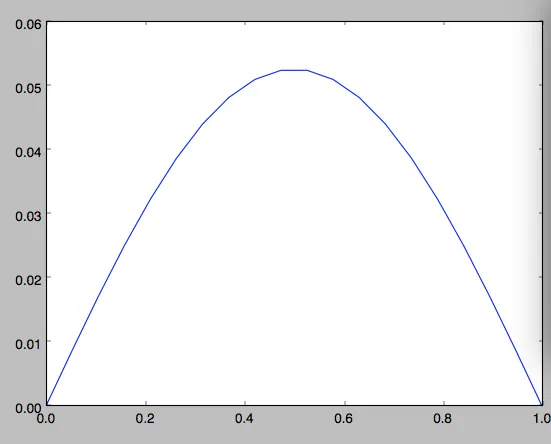 AU在x=0到x=1范围内(例如20个节点)给出以下绘图:
 然后我需要将U插值为更长的向量,并找到AU(对于更大的A也是如此,但不插值)。我通过以下方式进行插值:
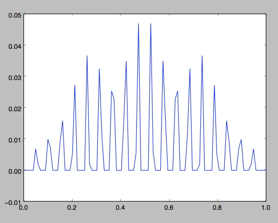
直到我将其与更长的A矩阵相乘,看起来都运行正常:
,将其转换为矩阵系统AU=F,其中A是刚度向量,解出U(对我的问题不是非常重要)。现在我已经得到了近似的U,在计算AU时应该得到类似F的向量,其中F为:
AU在x=0到x=1范围内(例如20个节点)给出以下绘图:
然后我需要将U插值为更长的向量,并找到AU(对于更大的A也是如此,但不插值)。我通过以下方式进行插值:U_inter = interp1d(x,U)
U_rich = U_inter(longer_x)
直到我将其与更长的A矩阵相乘,看起来都运行正常:
import numpy as np
import math
import scipy
from scipy.sparse import diags
import scipy.sparse.linalg
from scipy.interpolate import interp1d
import matplotlib
import matplotlib.pyplot as plt

def Poisson_Stiffness(x0):
    """Finds the Poisson equation stiffness matrix with any non uniform mesh x0"""

    x0 = np.array(x0)
    N = len(x0) - 1 # The amount of elements; x0, x1, ..., xN

    h = x0[1:] - x0[:-1]

    a = np.zeros(N+1)
    a[0] = 1 #BOUNDARY CONDITIONS
    a[1:-1] = 1/h[1:] + 1/h[:-1]
    a[-1] = 1/h[-1]
    a[N] = 1 #BOUNDARY CONDITIONS

    b = -1/h
    b[0] = 0 #BOUNDARY CONDITIONS

    c = -1/h
    c[N-1] = 0 #BOUNDARY CONDITIONS: DIRICHLET

    data = [a.tolist(), b.tolist(), c.tolist()]
    Positions = [0, 1, -1]
    Stiffness_Matrix = diags(data, Positions, (N+1,N+1))

    return Stiffness_Matrix

def NodalQuadrature(x0):
    """Finds the Nodal Quadrature Approximation of sin(pi x)"""

    x0 = np.array(x0)
    h = x0[1:] - x0[:-1]
    N = len(x0) - 1

    approx = np.zeros(len(x0))
    approx[0] = 0 #BOUNDARY CONDITIONS

    for i in range(1,N):
        approx[i] = math.sin(math.pi*x0[i])
        approx[i] = (approx[i]*h[i-1] + approx[i]*h[i])/2

    approx[N] = 0 #BOUNDARY CONDITIONS

    return approx

def Solver(x0):

    Stiff_Matrix = Poisson_Stiffness(x0)

    NodalApproximation = NodalQuadrature(x0)
    NodalApproximation[0] = 0

    U = scipy.sparse.linalg.spsolve(Stiff_Matrix, NodalApproximation)

    return U

x = np.linspace(0,1,10)
rich_x = np.linspace(0,1,50)
U = Solver(x)
A_rich = Poisson_Stiffness(rich_x)
U_inter = interp1d(x,U)
U_rich = U_inter(rich_x)
AUrich = A_rich.dot(U_rich)
plt.plot(rich_x,AUrich)
plt.show()
interp1d),那在哪里呢? - user707650