在R中按组引导结果向量

7

问题: 我如何使用 bootstrap 方法为数据帧中每个组(因子水平)计算的协方差矩阵的特征值上的一系列统计量获取置信区间?

问题描述: 我无法确定我需要的数据结构以便在boot函数中包含这些结果,或者一种“映射”bootstrap方法到各个组,并获得适合绘图的置信区间的方法。

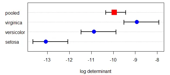
背景说明: 在heplots软件包中,boxM函数计算协方差矩阵相等的 Box's M 测试。该软件包提供了一个绘图函数可以绘制用于该测试的对数行列式的有用图形。该图形中的置信区间基于渐近理论逼近所得。

> library(heplots)
> iris.boxm <- boxM(iris[, 1:4], iris[, "Species"])
> iris.boxm

        Box's M-test for Homogeneity of Covariance Matrices

data:  iris[, 1:4]
Chi-Sq (approx.) = 140.94, df = 20, p-value < 2.2e-16

> plot(iris.boxm, gplabel="Species")

鸢尾花数据的对数行列式图

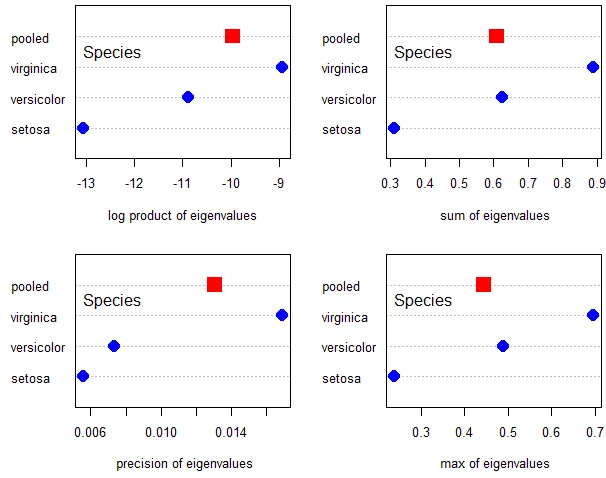
plot方法还可以显示特征值的其他函数,但在这种情况下没有可用的理论置信区间。

op <- par(mfrow=c(2,2), mar=c(5,4,1,1))
plot(iris.boxm, gplabel="Species", which="product")
plot(iris.boxm, gplabel="Species", which="sum")
plot(iris.boxm, gplabel="Species", which="precision")
plot(iris.boxm, gplabel="Species", which="max")
par(op)

在此输入图片描述

因此,我希望能够使用一种引导方法来计算这些置信区间,并在相应的图中显示它们。

我尝试过的方法:

以下是引导这些统计量的函数,但仅针对整个样本,而不考虑组 (Species)。

cov_stat_fun <- function(data, indices, 
            stats=c("logdet", "prod", "sum", "precision", "max")
            ) {
    dat <- data[indices,]
    cov <- cov(dat, use="complete.obs")
    eigs <- eigen(cov)$values

    res <- c(
        "logdet" = log(det(cov)),
        "prod" = prod(eigs),
        "sum" = sum(eigs),
        "precision" = 1/ sum(1/eigs),
        "max" = max(eigs)
        )
}

boot_cov_stat <- function(data, R=500,  ...) {
    boot(data, cov_stat_fun, R=R,  ...)
}

这个方法是可行的,但我需要按组别(以及总样本)来获取结果。
> iris.boot <- boot_cov_stat(iris[,1:4])
>
> iris.ci <- boot.ci(iris.boot)
> iris.ci
BOOTSTRAP CONFIDENCE INTERVAL CALCULATIONS
Based on 500 bootstrap replicates

CALL : 
boot.ci(boot.out = iris.boot)

Intervals : 
Level      Normal              Basic             Studentized     
95%   (-6.622, -5.702 )   (-6.593, -5.653 )   (-6.542, -5.438 )  

Level     Percentile            BCa          
95%   (-6.865, -5.926 )   (-6.613, -5.678 )  
Calculations and Intervals on Original Scale
Some BCa intervals may be unstable
>

我还编写了一个函数,用于计算每个组的单独协方差矩阵,但我不知道如何在我的自助函数中使用它。有人能帮忙吗?

# calculate covariance matrices by group and pooled
covs <- function(Y, group) {
   Y <- as.matrix(Y)
   gname <- deparse(substitute(group))
   if (!is.factor(group)) group <- as.factor(as.character(group))

   valid <- complete.cases(Y, group)
   if (nrow(Y) > sum(valid)) 
      warning(paste(nrow(Y) - sum(valid)), " cases with missing data have been removed.")
   Y <- Y[valid,]
   group <- group[valid]
   nlev <- nlevels(group)
   lev <- levels(group)
   mats <- aux <- list()
   for(i in 1:nlev) {
      mats[[i]] <- cov(Y[group == lev[i], ])
   }
   names(mats) <- lev
   pooled <- cov(Y)
   c(mats, "pooled"=pooled)
}

编辑: 在一个似乎相关的问题中,按组引导,建议使用boot()中的strata参数提供答案,但是没有展示它所给出的示例。[啊:仅确保在引导样本中以与数据中其频率相关的方式表示层次结构的strata参数。]

对于我的问题尝试这个,我并没有得到更多启示,因为我想要获取的是每个Species单独置信区间。

> iris.boot.strat <- boot_cov_stat(iris[,1:4], strata=iris$Species)
> 
> boot.ci(iris.boot.strat, conf=0.95, type=c("basic", "bca"))
BOOTSTRAP CONFIDENCE INTERVAL CALCULATIONS
Based on 500 bootstrap replicates

CALL : 
boot.ci(boot.out = iris.boot.strat, conf = 0.95, type = c("basic", 
    "bca"))

Intervals : 
Level      Basic                BCa          
95%   (-6.587, -5.743 )   (-6.559, -5.841 )  
Calculations and Intervals on Original Scale
Some BCa intervals may be unstable
> 
2个回答

4

如果我理解你的问题,你可以通过以下方式按组运行你的bootstrap函数:

library(boot)
library(tidyverse)

# Pooled
iris.boot <- boot_cov_stat(iris[,1:4])
iris.ci <- boot.ci(iris.boot)

# By Species
boot.list = setNames(unique(iris$Species), unique(iris$Species)) %>% 
  map(function(group) {
    iris.boot = boot_cov_stat(iris[iris$Species==group, 1:4])
    boot.ci(iris.boot)
  })

# Combine pooled and by-Species results
boot.list = c(boot.list, list(Pooled=iris.ci))

boot.list
$setosa
BOOTSTRAP CONFIDENCE INTERVAL CALCULATIONS
Based on 500 bootstrap replicates

CALL : 
boot.ci(boot.out = iris.boot)

Intervals : 
Level      Normal              Basic             Studentized     
95%   (-13.69, -11.86 )   (-13.69, -11.79 )   (-13.52, -10.65 )  

Level     Percentile            BCa          
95%   (-14.34, -12.44 )   (-13.65, -11.99 )  
Calculations and Intervals on Original Scale
Warning : BCa Intervals used Extreme Quantiles
Some BCa intervals may be unstable

$versicolor
BOOTSTRAP CONFIDENCE INTERVAL CALCULATIONS
Based on 500 bootstrap replicates

CALL : 
boot.ci(boot.out = iris.boot)

Intervals : 
Level      Normal              Basic             Studentized     
95%   (-11.37,  -9.81 )   (-11.36,  -9.78 )   (-11.25,  -8.97 )  

Level     Percentile            BCa          
95%   (-11.97, -10.39 )   (-11.35, -10.09 )  
Calculations and Intervals on Original Scale
Warning : BCa Intervals used Extreme Quantiles
Some BCa intervals may be unstable

$virginica
BOOTSTRAP CONFIDENCE INTERVAL CALCULATIONS
Based on 500 bootstrap replicates

CALL : 
boot.ci(boot.out = iris.boot)

Intervals : 
Level      Normal              Basic             Studentized     
95%   (-9.467, -7.784 )   (-9.447, -7.804 )   (-9.328, -6.959 )  

Level     Percentile            BCa          
95%   (-10.050,  -8.407 )   ( -9.456,  -8.075 )  
Calculations and Intervals on Original Scale
Warning : BCa Intervals used Extreme Quantiles
Some BCa intervals may be unstable

$Pooled
BOOTSTRAP CONFIDENCE INTERVAL CALCULATIONS
Based on 500 bootstrap replicates

CALL : 
boot.ci(boot.out = iris.boot)

Intervals : 
Level      Normal              Basic             Studentized     
95%   (-6.620, -5.714 )   (-6.613, -5.715 )   (-6.556, -5.545 )  

Level     Percentile            BCa          
95%   (-6.803, -5.906 )   (-6.624, -5.779 )  
Calculations and Intervals on Original Scale
Some BCa intervals may be unstable

这看起来非常准确。我现在正在参加一个会议,无法立即测试它。为了提供一个自包含的、规范的答案,我将接受并授予奖励,你能否编辑你的答案,同时显示使用类似
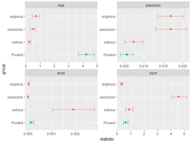
broom::tidy(boot.list)的东西的结果,即作为可用于绘图的数据框的结果。 - user101089
“broom” 没有整理 “bootci” 对象的方法,但我今天稍后会想办法解决。 - eipi10
好的,我会接受你的努力并授予赏金。 - user101089

1
我认为最好的一般性答案将是扩展@eipi10提出的方法,使用某种方法从bootci对象中提取所需的置信区间。这在broom包中缺失。
作为一种有益的替代方案,我尝试直接在引导结果上使用broom::tidy()。与(通常不对称的)置信区间不同,它给出了引导估计值作为statistic,一个bias和一个std.error。然而,从我得到的结果(见下文),我对broom::tidy()在这种情况下是否给出正确的结果表示怀疑。
# try just using tidy on the bootstrap results

## pooled
iris.boot <- boot_cov_stat(iris[,1:4])
iris.pooled <- tidy(iris.boot)

给予:
> iris.pooled
       term   statistic          bias    std.error
1    logdet -6.25922391 -0.0906294902 0.2469587430
2      prod  0.00191273 -0.0001120317 0.0004485317
3       sum  4.57295705 -0.0382145128 0.2861790776
4 precision  0.01692092 -0.0005047993 0.0016818910
5       max  4.22824171 -0.0329408193 0.2815648589
> 

现在,使用其他答案中描述的方法将此方法映射到组上,并进行合并:
## individual groups
boot.list2 = setNames(unique(iris$Species), unique(iris$Species)) %>% 
  map(function(group) {
    iris.boot = boot_cov_stat(iris[iris$Species==group, 1:4])
    tidy(iris.boot)
  })

# Combine pooled and by-Species results
boot.list <- c(boot.list2, list(Pooled=iris.pooled))

将其转换为数据框:
## transform this list to a data frame, with a group variable
result <- bind_rows(boot.list) %>% 
    mutate(group = rep(c( levels(iris$Species), "Pooled"), 5)) %>%
    arrange(term)

> result
        term     statistic          bias    std.error      group
1     logdet -1.306736e+01 -3.240621e-01 4.660334e-01     setosa
2     logdet -1.087433e+01 -2.872073e-01 3.949917e-01 versicolor
3     logdet -8.927058e+00 -2.925485e-01 4.424367e-01  virginica
4     logdet -6.259224e+00 -9.062949e-02 2.469587e-01     Pooled
5        max  2.364557e-01 -6.696719e-03 4.426305e-02     setosa
6        max  4.878739e-01 -6.798321e-03 8.662880e-02 versicolor
7        max  6.952548e-01 -6.517223e-03 1.355433e-01  virginica
8        max  4.228242e+00 -3.294082e-02 2.815649e-01     Pooled
9  precision  5.576122e-03 -5.928678e-04 8.533907e-04     Pooled
10 precision  7.338788e-03 -6.894908e-04 1.184594e-03     setosa
11 precision  1.691212e-02 -1.821494e-03 2.000718e-03 versicolor
12 precision  1.692092e-02 -5.047993e-04 1.681891e-03  virginica
13      prod  2.113088e-06 -4.158518e-07 7.850009e-07 versicolor
14      prod  1.893828e-05 -3.605691e-06 6.100376e-06  virginica
15      prod  1.327479e-04 -2.381536e-05 4.792428e-05     Pooled
16      prod  1.912730e-03 -1.120317e-04 4.485317e-04     setosa
17       sum  3.092041e-01 -1.005543e-02 4.623437e-02  virginica
18       sum  6.248245e-01 -1.238896e-02 8.536621e-02     Pooled
19       sum  8.883673e-01 -1.500578e-02 1.409230e-01     setosa
20       sum  4.572957e+00 -3.821451e-02 2.861791e-01 versicolor
> 

这样可以得到一个可以绘制的东西,据说对应于原始问题中显示的没有误差条的图形:
result %>% mutate(Pooled = group == "Pooled") %>%
    filter (term != "logdet") %>%
    ggplot(aes(y=statistic, x=group, color=Pooled)) +
    geom_point(size=2.5) +
    geom_errorbar(aes(ymin=statistic-2*std.error, 
                      ymax=statistic+2*std.error), width=0.4) +
    facet_wrap( ~ term, scales="free") +
    coord_flip() + guides(color=FALSE)

enter image description here

然而,这个“整洁的图表”似乎明显是错误的。理论上说,对于Polled样本的结果必须在每种情况下都介于单独组的结果之间,因为它在某种程度上是组合凸包。将下面的图表与原始问题中给出的进行比较。(可能我在这里做错了什么,但我看不出有什么缺陷。)

网页内容由stack overflow 提供, 点击上面的
可以查看英文原文,
原文链接