XOR神经网络反向传播

Question

XOR神经网络反向传播

pythonmachine-learningneural-networkbackpropagation

3

我在Python中尝试实现一个基本的带有1个隐藏层的XOR神经网络。特别是，我没有理解反向传播算法，所以一直卡在计算delta2和更新权重上...能帮帮我吗？

import numpy as np

def sigmoid(x):
    return 1.0 / (1.0 + np.exp(-x))

vec_sigmoid = np.vectorize(sigmoid)

theta1 = np.matrix(np.random.rand(3,3))
theta2 = np.matrix(np.random.rand(3,1))

def fit(x, y, theta1, theta2, learn_rate=.001):
    #forward pass
    layer1 = np.matrix(x, dtype='f')
    layer1 = np.c_[np.ones(1), layer1]
    layer2 = vec_sigmoid(layer1*theta1)
    layer3 = sigmoid(layer2*theta2)

    #backprop
    delta3 = y - layer3
    delta2 = (theta2*delta3) * np.multiply(layer2, 1 - layer2) #??

    #update weights
    theta2 += learn_rate * delta3 #??
    theta1 += learn_rate * delta2 #??

def train(X, Y):
    for _ in range(10000):
        for i in range(4):
            x = X[i]
            y = Y[i]
            fit(x, y, theta1, theta2)


X = [(0,0), (1,0), (0,1), (1,1)]
Y = [0, 1, 1, 0]    
train(X, Y)

- WBC

1个回答

网页内容由stack overflow 提供, 点击上面的

可以查看英文原文，
原文链接

- bnsh · Accepted Answer

好的，首先，这是修改后的代码，可以使您的代码正常运行。

#! /usr/bin/python

import numpy as np

def sigmoid(x):
    return 1.0 / (1.0 + np.exp(-x))

vec_sigmoid = np.vectorize(sigmoid)

# Binesh - just cleaning it up, so you can easily change the number of hiddens.
# Also, initializing with a heuristic from Yoshua Bengio.
# In many places you were using matrix multiplication and elementwise multiplication
# interchangably... You can't do that.. (So I explicitly changed everything to be
# dot products and multiplies so it's clear.)
input_sz = 2;
hidden_sz = 3;
output_sz = 1;
theta1 = np.matrix(0.5 * np.sqrt(6.0 / (input_sz+hidden_sz)) * (np.random.rand(1+input_sz,hidden_sz)-0.5))
theta2 = np.matrix(0.5 * np.sqrt(6.0 / (hidden_sz+output_sz)) * (np.random.rand(1+hidden_sz,output_sz)-0.5))

def fit(x, y, theta1, theta2, learn_rate=.1):
    #forward pass
    layer1 = np.matrix(x, dtype='f')
    layer1 = np.c_[np.ones(1), layer1]
    # Binesh - for layer2 we need to add a bias term.
    layer2 = np.c_[np.ones(1), vec_sigmoid(layer1.dot(theta1))]
    layer3 = sigmoid(layer2.dot(theta2))

    #backprop
    delta3 = y - layer3
    # Binesh - In reality, this is the _negative_ derivative of the cross entropy function
    # wrt the _input_ to the final sigmoid function.

    delta2 = np.multiply(delta3.dot(theta2.T), np.multiply(layer2, (1-layer2)))
    # Binesh - We actually don't use the delta for the bias term. (What would be the point?
    # it has no inputs. Hence the line below.
    delta2 = delta2[:,1:]

    # But, delta's are just derivatives wrt the inputs to the sigmoid.
    # We don't add those to theta directly. We have to multiply these by
    # the preceding layer to get the theta2d's and theta1d's
    theta2d = np.dot(layer2.T, delta3)
    theta1d = np.dot(layer1.T, delta2)

    #update weights
    # Binesh - here you had delta3 and delta2... Those are not the
    # the derivatives wrt the theta's, they are the derivatives wrt
    # the inputs to the sigmoids.. (As I mention above)
    theta2 += learn_rate * theta2d #??
    theta1 += learn_rate * theta1d #??

def train(X, Y):
    for _ in range(10000):
        for i in range(4):
            x = X[i]
            y = Y[i]
            fit(x, y, theta1, theta2)


# Binesh - Here's a little test function to see that it actually works
def test(X):
    for i in range(4):
        layer1 = np.matrix(X[i],dtype='f')
        layer1 = np.c_[np.ones(1), layer1]
        layer2 = np.c_[np.ones(1), vec_sigmoid(layer1.dot(theta1))]
        layer3 = sigmoid(layer2.dot(theta2))
        print "%d xor %d = %.7f" % (layer1[0,1], layer1[0,2], layer3[0,0])

X = [(0,0), (1,0), (0,1), (1,1)]
Y = [0, 1, 1, 0]    
train(X, Y)

# Binesh - Alright, let's see!
test(X)

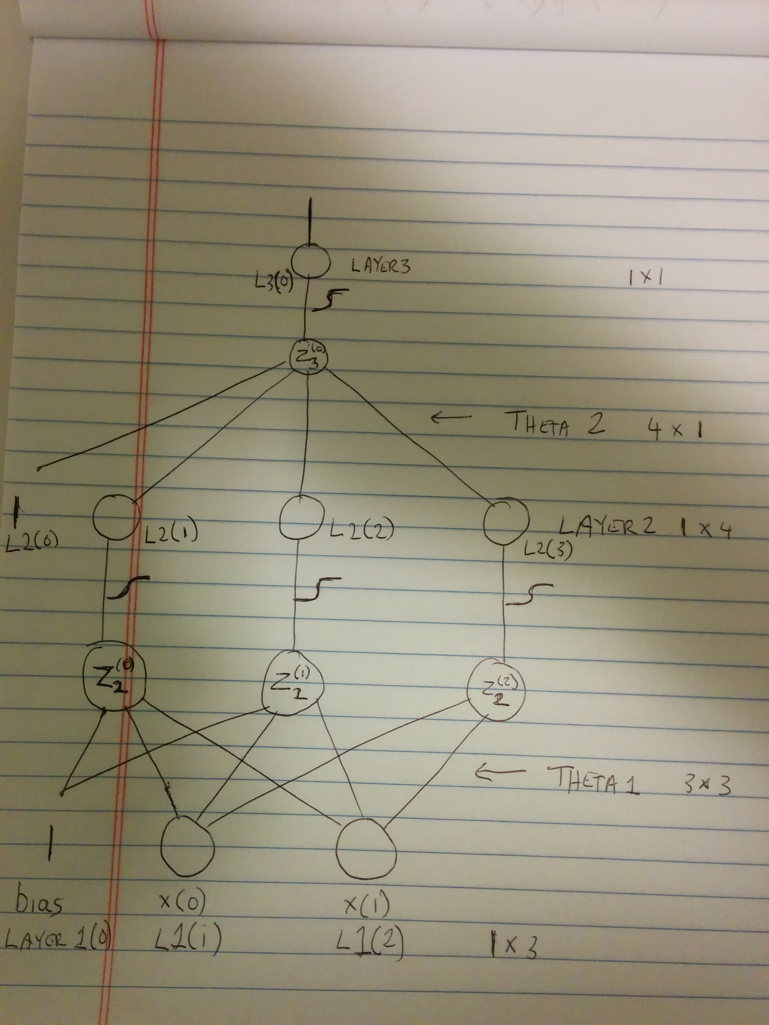
现在解释一下。请原谅这个简陋的图示。拍照比在gimp中画东西更容易。

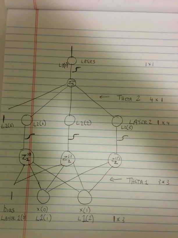
_{(来源：cablemodem.hex21.com上的binesh)}

所以，首先我们有误差函数。我们将其称为CE（交叉熵）。我会尽可能使用您的变量，但我将使用L1、L2和L3代替layer1、layer2和layer3。叹息（我不知道如何在这里使用latex。它似乎在统计堆栈交换中起作用。奇怪。）

CE = -(Y log(L3) + (1-Y) log(1-L3))

我们需要对此关于 L3 求导，这样我们就能看到如何移动 L3 以便减小这个值。

dCE/dL3 = -((Y/L3) - (1-Y)/(1-L3))
        = -((Y(1-L3) - (1-Y)L3) / (L3(1-L3)))
        = -(((Y-Y*L3) - (L3-Y*L3)) / (L3(1-L3)))
        = -((Y-Y3*L3 + Y3*L3 - L3) / (L3(1-L3)))
        = -((Y-L3) / (L3(1-L3)))
        = ((L3-Y) / (L3(1-L3)))

很好，但实际上，我们不能随意更改L3。L3是Z3的函数（见我的图片）。

L3      = sigmoid(Z3)
dL3/dZ3 = L3(1-L3)

我这里不会推导sigmoid函数的导数，但其实证明并不那么难。

无论如何，这就是L3对Z3的导数，但我们想要CE对Z3的导数。

dCE/dZ3 = (dCE/dL3) * (dL3/dZ3)
        = ((L3-Y)/(L3(1-L3)) * (L3(1-L3)) # Hey, look at that. The denominator gets cancelled out and
        = (L3-Y) # This is why in my comments I was saying what you are computing is the _negative_ derivative.

我们把对Z求导数叫做“delta”。所以，在你的代码中，这对应着delta3。

很好，但是我们不能随意改变Z3。我们需要计算它相对于L2的导数。

但这更加复杂。

Z3 = theta2(0) + theta2(1) * L2(1) + theta2(2) * L2(2) + theta2(3) * L2(3)

因此，我们需要对L2（1），L2（2）和L2（3）进行偏导数计算。

dZ3/dL2(1) = theta2(1)
dZ3/dL2(2) = theta2(2)
dZ3/dL2(3) = theta2(3)

请问是否需要将以下内容一并翻译？如果需要，请提供完整的HTML代码。谢谢！

dZ3/dBias  = theta2(0)

但是偏差永远不会改变，它始终为1，因此我们可以放心地忽略它。但是，我们的第二层包括偏差，所以现在我们将保留它。

但是，我们再次想要关于Z2(0), Z2(1), Z2(2)的导数（看起来我画得不太好，很遗憾。请看图表，我认为这样更清楚。）

dL2(1)/dZ2(0) = L2(1) * (1-L2(1))
dL2(2)/dZ2(1) = L2(2) * (1-L2(2))
dL2(3)/dZ2(2) = L2(3) * (1-L2(3))

现在的dCE/dZ2(0..2)是什么？

dCE/dZ2(0) = dCE/dZ3 * dZ3/dL2(1) * dL2(1)/dZ2(0)
           = (L3-Y)  * theta2(1)  * L2(1) * (1-L2(1))

dCE/dZ2(1) = dCE/dZ3 * dZ3/dL2(2) * dL2(2)/dZ2(1)
           = (L3-Y)  * theta2(2)  * L2(2) * (1-L2(2))

dCE/dZ2(2) = dCE/dZ3 * dZ3/dL2(3) * dL2(3)/dZ2(2)
           = (L3-Y)  * theta2(3)  * L2(3) * (1-L2(3))

但是，实际上我们可以将其表达为（delta3 * Transpose [theta2]）逐元素乘以（L2 *（1-L2））（其中L2是向量）

这些是我们的delta2层。我删除了它的第一个条目，因为如我上面所提到的，它对应于偏置的delta（我在图表中标记为L2（0））。

现在，我们已经得到了关于Z的导数，但是我们只能修改我们的thetas。

Z3 = theta2(0) + theta2(1) * L2(1) + theta2(2) * L2(2) + theta2(3) * L2(3)
dZ3/dtheta2(0) = 1
dZ3/dtheta2(1) = L2(1)
dZ3/dtheta2(2) = L2(2)
dZ3/dtheta2(3) = L2(3)

再次强调，我们需要求出dCE/dtheta2(0)，因此变成了：

dCE/dtheta2(0) = dCE/dZ3 * dZ3/dtheta2(0)
               = (L3-Y) * 1
dCE/dtheta2(1) = dCE/dZ3 * dZ3/dtheta2(1)
               = (L3-Y) * L2(1)
dCE/dtheta2(2) = dCE/dZ3 * dZ3/dtheta2(2)
               = (L3-Y) * L2(2)
dCE/dtheta2(3) = dCE/dZ3 * dZ3/dtheta2(3)
               = (L3-Y) * L2(3)

好的，这只是np.dot(layer2.T, delta3)的简写，而这正是我在theta2d中拥有的内容

同样地： Z2(0) = theta1(0,0) + theta1(1,0) * L1(1) + theta1(2,0) * L1(2) dZ2(0)/dtheta1(0,0) = 1 dZ2(0)/dtheta1(1,0) = L1(1) dZ2(0)/dtheta1(2,0) = L1(2)

Z2(1) = theta1(0,1) + theta1(1,1) * L1(1) + theta1(2,1) * L1(2)
dZ2(1)/dtheta1(0,1) = 1
dZ2(1)/dtheta1(1,1) = L1(1)
dZ2(1)/dtheta1(2,1) = L1(2)

Z2(2) = theta1(0,2) + theta1(1,2) * L1(1) + theta1(2,2) * L1(2)
dZ2(2)/dtheta1(0,2) = 1
dZ2(2)/dtheta1(1,2) = L1(1)
dZ2(2)/dtheta1(2,2) = L1(2)

同时，我们需要乘以dCE/dZ2(0)，dCE/dZ2(1)和dCE/dZ2(2)（对于上面的每个三组）。但是，如果你考虑一下，那么这就变成了np.dot(layer1.T, delta2)，这就是我在theta1d中的内容。

现在，因为你在代码中使用了Y-L3，所以你正在将theta1和theta2相加...但是，这里的推理是什么？我们刚刚计算出来的是CE wrt权重的导数。因此，这意味着增加权重将会增加CE。但是，我们真正想要减少CE。因此，我们要进行减法（通常情况下）。但是，由于在你的代码中，你正在计算负导数，所以添加是正确的。

这有意义吗？