绘制套索回归的beta系数图

Question

绘制套索回归的beta系数图

rmachine-learningregressionglmnetlasso-regression

4

我用R语言编写了这段Lasso代码，并得到了一些Beta值：

#Lasso
library(MASS)
library(glmnet)
Boston=na.omit(Boston)
x=model.matrix(crim~.,Boston)[,-1]
rownames(x)=c()
y=as.matrix(Boston$crim)
lasso.mod =glmnet(x,y, alpha =1, lambda = 0.1)
beta=as.matrix(rep(0,19))
beta=coef(lasso.mod)
matplot(beta,type="l",lty=1,xlab="L1",ylab="beta",main="lasso")

我想绘制一个像这样的图表来表示贝塔值：

enter image description here

但是我不知道在R中可以使用哪个绘图函数来完成。

- Majk

1

我认为plot(lasso.mod)可以实现这个功能，请提供数据集以使示例可重现（可能从r包中加载？） - Gilles San Martin

@Gilles 我仍然添加了*library(MASS)*来使用数据集。这是链接下载它。我实际上想知道如何在不使用lasso.mod的情况下绘制beta值的图表。 - Majk

1

如果您想查看不同正则化水平下系数的值，也不应该固定lambda: lasso.mod =glmnet(x,y, alpha =1)，然后使用coef(lasso.mod)和/或plot(lasso.mod)。 - Gilles San Martin

@Gilles 谢谢，但是有没有办法像 plot(beta) 这样绘制贝塔值，而不必执行 plot(lasso.mod)？ - Majk

典型的交叉验证/stats问题。已标记为需要移动到那里。 - ZF007

1个回答

网页内容由stack overflow 提供, 点击上面的

可以查看英文原文，
原文链接

- Gilles San Martin · Accepted Answer

我不明白为什么你不想使用内置的glmnet方法，但你肯定可以复制它的结果（这里使用ggplot）。
你仍然需要模型对象来提取lambda值...

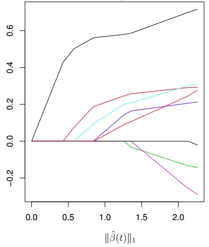
编辑：添加了系数与L1范数

复制您的最小示例

library(MASS)
library(glmnet)
#> Le chargement a nécessité le package : Matrix
#> Le chargement a nécessité le package : foreach
#> Loaded glmnet 2.0-13
library(ggplot2)
library(reshape)
#> 
#> Attachement du package : 'reshape'
#> The following object is masked from 'package:Matrix':
#> 
#>     expand

Boston=na.omit(Boston)
x=model.matrix(crim~.,Boston)[,-1]
y=as.matrix(Boston$crim)
lasso.mod =glmnet(x,y, alpha =1)
beta=coef(lasso.mod)

提取coef值并将它们转换为适合于ggplot的长格式整洁形式。

tmp <- as.data.frame(as.matrix(beta))
tmp$coef <- row.names(tmp)
tmp <- reshape::melt(tmp, id = "coef")
tmp$variable <- as.numeric(gsub("s", "", tmp$variable))
tmp$lambda <- lasso.mod$lambda[tmp$variable+1] # extract the lambda values
tmp$norm <- apply(abs(beta[-1,]), 2, sum)[tmp$variable+1] # compute L1 norm

使用ggplot绘制图表：coef vs lambda

# x11(width = 13/2.54, height = 9/2.54)
ggplot(tmp[tmp$coef != "(Intercept)",], aes(lambda, value, color = coef, linetype = coef)) + 
    geom_line() + 
    scale_x_log10() + 
    xlab("Lambda (log scale)") + 
    guides(color = guide_legend(title = ""), 
           linetype = guide_legend(title = "")) +
    theme_bw() + 
    theme(legend.key.width = unit(3,"lines"))

使用glmnet基本绘图方法是相同的：

# x11(width = 9/2.54, height = 8/2.54)
par(mfrow = c(1,1), mar = c(3.5,3.5,2,1), mgp = c(2, 0.6, 0), cex = 0.8, las = 1)
plot(lasso.mod, "lambda", label = TRUE)

使用ggplot绘制图表：coef vs L1 norm

# x11(width = 13/2.54, height = 9/2.54)
ggplot(tmp[tmp$coef != "(Intercept)",], aes(norm, value, color = coef, linetype = coef)) + 
    geom_line() + 
    xlab("L1 norm") + 
    guides(color = guide_legend(title = ""), 
           linetype = guide_legend(title = "")) +
    theme_bw() + 
    theme(legend.key.width = unit(3,"lines"))

对于基本的glmnet方法，情况是相同的：

# x11(width = 9/2.54, height = 8/2.54)
par(mfrow = c(1,1), mar = c(3.5,3.5,2,1), mgp = c(2, 0.6, 0), cex = 0.8, las = 1)
plot(lasso.mod, "norm", label = TRUE)

此内容是由reprex包（v0.2.0）于2018年2月26日创建的。