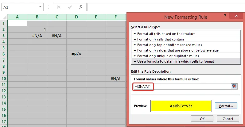
如何在VBA中填充单元格颜色？

Question

我想在当前工作表中对值为“＃N/A”的单元格进行着色。 为了实现此目的，我使用以下宏：

Sub ColorCells()

Dim Data As Range
Dim cell As Range
Set currentsheet = ActiveWorkbook.Sheets("Comparison")
Set Data = currentsheet.Range("A2:AW1048576")

For Each cell In Data
If cell.Value = "#N/A" Then
   cell.Interior.ColorIndex = 3
End If
Next

End Sub

但是这行代码If cell.Value = "#N/A" Then会出现错误：类型不匹配。也许有人可以帮忙理解一下哪里出错了？谢谢。

- Ale

---

为什么不使用条件格式突出显示有错误的单元格？如果您不喜欢这种方法，请使用 If cell.Text ="#N/A" Then。还有一个提示，尝试使用 Set Data = Intersect(currentsheet.UsedRange,currentsheet.Range("A2:AW1048576")) 来最小化循环中的单元格数量。现在您正在遍历5000万个单元格 :) - Dmitry Pavliv

你也可以使用 IsError(Cell.Value)。 - Kapol

使用.text代替.value - Sathish Kothandam

Answer 1

无需使用VBA的解决方案：

使用条件格式公式：=ISNA(A1)（用于突出显示所有错误单元格-不仅限于#N/A，使用=ISERROR(A1)以突出显示所有错误）

使用VBA的解决方案：

您的代码循环遍历5000万个单元格。为了减少单元格数量，我使用.SpecialCells(xlCellTypeFormulas, 16)和.SpecialCells(xlCellTypeConstants, 16)只返回带有错误的单元格（请注意，我使用If cell.Text = "#N/A" Then）

Sub ColorCells()
    Dim Data As Range, Data2 As Range, cell As Range
    Dim currentsheet As Worksheet

    Set currentsheet = ActiveWorkbook.Sheets("Comparison")

    With currentsheet.Range("A2:AW" & Rows.Count)
        .Interior.Color = xlNone
        On Error Resume Next
        'select only cells with errors
        Set Data = .SpecialCells(xlCellTypeFormulas, 16)
        Set Data2 = .SpecialCells(xlCellTypeConstants, 16)
        On Error GoTo 0
    End With

    If Not Data2 Is Nothing Then
        If Not Data Is Nothing Then
            Set Data = Union(Data, Data2)
        Else
            Set Data = Data2
        End If
    End If

    If Not Data Is Nothing Then
        For Each cell In Data
            If cell.Text = "#N/A" Then
               cell.Interior.ColorIndex = 4
            End If
        Next
    End If
End Sub

注意，要突出显示任何错误的单元格（不仅限于"#N/A"），请替换以下代码

If Not Data Is Nothing Then
   For Each cell In Data
       If cell.Text = "#N/A" Then
          cell.Interior.ColorIndex = 3
       End If
   Next
End If

If Not Data Is Nothing Then Data.Interior.ColorIndex = 3

更新：（如何通过 VBA 添加CF规则）

Sub test()
    With ActiveWorkbook.Sheets("Comparison").Range("A2:AW" & Rows.Count).FormatConditions
        .Delete
        .Add Type:=xlExpression, Formula1:="=ISNA(A1)"
        .Item(1).Interior.ColorIndex = 3
    End With
End Sub

- Dmitry Pavliv

---

谢谢！两种方法都可以正常工作！使用VBA的唯一问题是，如果我需要使用另一个输入运行宏，并且N/A单元格的位置发生更改，则此宏不会重写颜色。例如，如果A2单元格被着色，则即使从第二次尝试开始不再有N/A值，它仍然保持着色状态。 - Ale

@Ale，在这种情况下，请在“On Error Resume Next”之前添加以下行：currentsheet.Range("A2:AW" & Rows.Count).Interior.Color = xlNone（请参见我的更新答案）。 - Dmitry Pavliv

可能需要将A列始终涂成灰色，但B列包含一些值和N/A，需要涂成红色。包含N/A的单元格取决于输入文件和另一个宏。因此，如果N/A位置发生变化，我必须清除以前的红色，但仍然保留A列的灰色。但在这种情况下，最好使用CF。谢谢！ - Ale

@Ale，请看一下我的更新部分，关于如何通过VBA创建CF规则 :) - Dmitry Pavliv

谢谢，它运行得很好！但是我实际上录制了一个执行CF的宏，所以VBA自动创建了命令。 :) - Ale

Answer 2

1. Use conditional formatting instead of VBA to highlight errors.

2. Using a VBA loop like the one you posted will take a long time to process

3. the statement If cell.Value = "#N/A" Then will never work. If you insist on using VBA to highlight errors, try this instead.

   Sub ColorCells()

   Dim Data As Range
   Dim cell As Range
   Set currentsheet = ActiveWorkbook.Sheets("Comparison")
   Set Data = currentsheet.Range("A2:AW1048576")
   
   For Each cell In Data
   
   If IsError(cell.Value) Then
      cell.Interior.ColorIndex = 3
   End If
   Next
   
   End Sub
   

4. Be prepared for a long wait, since the procedure loops through 51 million cells

5. There are more efficient ways to achieve what you want to do. Update your question if you have a change of mind.

- teylyn

---

谢谢您！实际上我正在寻找VBA解决方案，但这个也可以。 - Ale

Answer 3

1. 通过左上角选择所有单元格
2. 选择[开始] >> [条件格式] >> [新建规则]
3. 选择[仅对包含内容的单元格设置格式]
4. 在[仅显示以下类型的单元格:]中选择"错误"
5. 点击[格式...]按钮选择适当的格式

- Alpha

Answer 4

你需要使用 cell.Text = "#N/A" 而不是 cell.Value = "#N/A"。单元格中的错误实际上只是存储在单元格中的文本。

- Dustin Knight