计算点到一条直线的垂直距离

Question

计算点到一条直线的垂直距离

r

4

注意不要与此帖子混淆。

与此帖子非常相似。

这是一个非常简单的概念。

我有一组点，想要计算每个点到一条线的法线距离。

在此可复现的示例中，我加载了sp::meuse数据并绘制了一条线。如何向meuse添加一列，使其等于每个点到该线法线(垂直)距离？

# load data
library(sp)
data(meuse)

# create new line
newline = data.frame(y = seq(from = 330000, to = 334000, length.out = 100), x = seq(from = 178000, to = 181000, length.out = 100))
# plot the data
meuse %>% 
  ggplot(aes(x, y)) + geom_point() + 
  ggtitle("Zinc Concentration (ppm)") + coord_equal() +
  geom_line(data = newline, aes(x,y))

为了举例说明：

- Rich Pauloo

可能是重复的问题：使用R，如何计算从一点到一条直线的距离？ - Chris Holbrook

@ChrisHolbrook，这个问题有两个不同之处。我正在寻找一组点到一条线的垂直距离。 - Rich Pauloo

2个回答

1

除了@Giles的答案，我想分享另一种方法，以防其他遇到同样问题的人阅读此内容。

以下两个函数接受由一系列点定义的线和另一组点，并计算每个点与该线之间的最小距离，如上所述。

1. 毕达哥拉斯定理：用于计算欧几里得直线距离（在球体上，如地球，这条直线会穿过地球）。除非是在二维平面上，否则不太正确。

# data for the function
line <- data.frame(x = seq(from = 178000, to = 181000, length.out = nrow(meuse)),
                   y = seq(from = 330000, to = 334000, length.out = nrow(meuse)))
data(meuse)
pts <- meuse[,1:2] # the pts must **only** be a set of x,y coords.

# takes a line defined by a set of points along a line, and a set of points, and
# returns the minimum (orthogonal) Euclidian distance between all pts and
# the line.
euclid_min_d <- function(line, pts){
  d <- vector(mode = "integer", length = nrow(pts))
  for(i in 1:nrow(pts)){
    d[i] = min(( abs(abs(pts$x[i]) - abs(line$x)) + abs(abs(pts$y[i]) - abs(line$y)) )^(.5))
  }
  return(d)
}

# run the function

> euclid_min_d(line, pts)
  [1] 19.100214 18.884131 22.751052 26.279714 28.542290 30.792561 25.281532 22.542312 25.311822 29.261029
 [11] 29.244158 27.581520 19.304464 23.133997 25.341819 19.891916 20.933723 21.650710 22.187513 23.017780
 [21] 24.815684 25.861519 26.623883 31.012356 32.121523 32.921197 30.427047 31.005236 29.177246 33.856458
 [31] 34.725454 31.817866 31.557616 34.042563 34.963060 31.055041 28.352833 25.067182 23.438231 23.029907
 [41] 27.357185 30.330645 28.661028 29.866152 25.177809 26.005244 27.847684 29.808262 31.489227 31.789895
 [51] 31.186702 21.838248 19.593930 16.820674 12.939921  8.453079 16.431282 17.929516 21.105486  8.029976
 [61]  8.775704 13.154921 16.281613 17.222758 17.667933 17.583567 25.114026 31.508193 35.387833 20.621827
 [71] 21.949470 20.537264 21.489955 23.383866 23.437953 24.926646 26.035939 17.687034 18.105391 17.051869
 [81] 18.006853 43.461582 18.294844 26.630712 22.386800 22.206820 19.229644 19.982785 22.110408 23.343288
 [91] 27.182643 17.403911 16.936858 36.972085 34.168034 31.318639 29.846360 26.406414 25.530730 30.197618
[101] 35.733501 37.126320 37.440689 34.361334 33.550698 36.716888 38.238826 39.461143 38.888285 34.671183
[111] 32.966138 28.270263 28.243376 25.291033 19.522880 18.844201 18.683280 45.283953 28.036386 27.277554
[121] 18.934611 13.435271 15.683145 23.364975 23.064562 31.654589 33.422133 32.795906 22.917696 23.211618
[131] 36.513118 27.062218 27.744895 34.663690 30.394377 29.861151 34.564827 26.293548 24.816469 27.611404
[141] 34.684103 37.463055 40.124805 40.472213 38.301436 39.127995 35.930488 31.048349 35.284558 31.208557
[151] 32.370020 29.511389 25.336181 34.386081 49.889358

2. `sp::spDist` 或 `sp::spDistN1`：Haversine（大圆）距离，适用于球体的曲面上。对于空间经纬度数据，特别是大范围的点，更加正确。

# Haversine (Great Circle distance) for spatial points
library(sp)

# bring in data
data(meuse)

# define a line by a sequence of points between two points at the ends of a line. 
# length can be any number. as length approaches infinity, the distance between 
# points and the line appraoches a normal (orthogonal) orientation

line <- data.frame(x = seq(from = 178000, to = 181000, length.out = nrow(meuse)),
                       y = seq(from = 330000, to = 334000, length.out = nrow(meuse)))

# columns 1 and 2 are long/lat, column 3 is extra data to make the SPDF
pts <- meuse[,1:3] 

# sp::spDists only takes spatial objects, so make line and pts 'spatial objects' 
coordinates(line) <- c("x","y")
coordinates(pts) <- c("x","y")
class(line) # spdf
class(pts) # spdf

# takes a line defined by a set of points along a line, and a set of points, and
# returns the minimum (orthogonal) Great circle distance between all pts and
# the line.

gc_min_d <- function(line, pts){
  d <- vector(mode = "integer", length = nrow(pts))
  for(i in 1:nrow(pts@coords)){
    d[i] = min(spDistsN1(line, pts@coords[i,]))
  }
  return(d)
}

# run the function

> gc_min_d(line, pts)
  [1]  291.11720  285.53973  409.96584  548.04129  647.62204  756.00049  510.23214  403.85051  509.42670
 [10]  684.83496  683.85902  607.07043  296.06328  424.00002  512.42695  316.53043  348.31645  372.00033
 [19]  391.95541  419.80867  489.01900  533.00685  564.94128  767.47913  823.85186  866.80035  740.20012
 [28]  766.21521  681.05998  914.12500  964.42709  809.15362  793.28237  923.85091  974.03591  770.16568
 [37]  638.61108  501.28887  435.72032  420.80271  597.42032  733.09464  655.81036  709.53065  504.62940
 [46]  539.63972  618.02925  709.00052  791.80007  804.61682  776.86267  379.10017  304.56883  225.40137
 [55]  131.15538   54.74886  212.76568  253.89445  352.36923   49.33170   59.28282  134.22712  211.55102
 [64]  234.80732  247.80522  245.84412  501.01377  793.84395 1001.00078  339.25067  382.25984  333.60141
 [73]  369.72499  433.24388  438.60154  494.40929  540.41364  248.70466  262.20469  230.42463  258.05366
 [82] 1509.07023  264.01918  566.03235  396.98188  393.42160  294.08301  317.21856  390.41809  433.23431
 [91]  586.86838  240.47441  226.83961 1090.66783  933.51589  783.80282  710.00866  556.40688  518.09206
[100]  726.00636 1019.61784 1101.62687 1120.26196  942.68793  897.40984 1077.08258 1167.68956 1243.01891
[109] 1209.40946  957.62977  866.73835  635.60151  637.89236  509.05787  303.69985  280.34209  277.20013
[118] 1637.20259  627.43972  591.21355  286.64675  141.47774  194.00723  434.05177  425.10718  801.54641
[127]  889.25788  857.64172  420.13830  430.81025 1064.83266  584.79094  614.02411  957.26008  738.60392
[136]  712.45532  951.40992  549.20351  490.60506  608.26798  961.20035 1121.64783 1276.01133 1271.80112
[145] 1147.71273 1167.60070  979.46392  735.61392  974.03783  774.80205  838.08370  692.84592  513.42862
[154]  944.32835 1987.61385

- Rich Pauloo

你是不是忘了对坐标差的平方进行计算？也就是说，在第一个情况下，我会这样写：d[i] = min(( abs(abs(pts$x[i]) - abs(line$x))^2 + abs(abs(pts$y[i]) - abs(line$y))^2 )^(.5)) - atsyplenkov

网页内容由stack overflow 提供, 点击上面的

可以查看英文原文，
原文链接

- Gilles San Martin · Accepted Answer

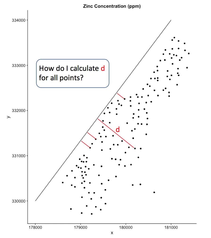
由于您正在使用meuse数据，因此使用空间对象和空间计算似乎是很自然的：

library(sf)
library(sp)
data(meuse)

# create new line - please note the small changes relative to your code : 
# x = first column and cbind to have a matrix instead of a data.frame
newline = cbind(x = seq(from = 178000, to = 181000, length.out = 100),
                y = seq(from = 330000, to = 334000, length.out = 100))

# transform the points and lines into spatial objects
meuse <- st_as_sf(meuse, coords = c("x", "y"))
newline <- st_linestring(newline)

# Compute the distance - works also for non straight lines !
st_distance(meuse, newline) [1:10]
## [1] 291.0 285.2 409.8 548.0 647.6 756.0 510.0 403.8 509.4 684.8


# Ploting to check that your line is were you expect it
plot_sf(meuse)
plot(meuse, add = TRUE)
plot(newline, add = TRUE)

您可以通过在仅有2个坐标的直线上运行相同的代码来证明这些是相对于您的直线的垂直距离。
但请注意，这是到直线的最短距离。因此，对于靠近线段端点或超出直线范围的点，您将无法得到垂直距离（只有到端点的最短距离）。
您必须有足够长的线以避免这种情况...

newline = cbind(x = c(178000, 181000), 
                y = c(330000, 334000))

# transform the points and lines into spatial objects
meuse <- st_as_sf(meuse, coords = c("x", "y"), crs = 31370)
newline <- st_linestring(newline)

# Compute the distance - works also for non straight lines !
st_distance(meuse, newline) [1:10]
## [1] 291.0 285.2 409.8 548.0 647.6 756.0 510.0 403.8 509.4 684.8


# Ploting to check that your line is were you expect it
plot_sf(meuse)
plot(meuse, add = TRUE)
plot(newline, add = TRUE)

如果直线的斜率为1，则可以使用勾股定理（x的差异= y的差异=到直线的距离/ sqrt(2)）计算点在直线上的投影。但是这里不适用（红色线段与直线不垂直），因为斜率不是1，因此y坐标的差异不等于x坐标的差异。勾股定理在这里无法解决。（但是由st_distance计算出的距离是垂直于直线的。）

distances <- st_distance(meuse, newline)
newline = data.frame(x = c(178000, 181000), 
                     y = c(330000, 334000))

segments <- as.data.frame(st_coordinates(meuse))
segments <- data.frame(
    segments, 
    X2 = segments$X - distances/sqrt(2), 
    Y2 = segments$Y + distances/sqrt(2)
)    

library(ggplot2)
ggplot() +
    geom_point(data = segments, aes(X,Y)) +
    geom_line(data = newline, aes(x,y)) +
    geom_segment(data = segments, aes(x = X, y = Y, xend = X2, yend = Y2), 
                 color = "orangered", alpha = 0.5) +
    coord_equal() + xlim(c(177000, 182000))

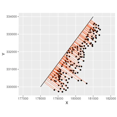
如果您只想绘制它，可以使用 rgeos 的 gProject 函数(目前在sf中没有等价函数)来获取点在线上投影的坐标。您需要将点和线以ssp格式而不是sf格式提供，并在 sp 的矩阵和 ggplot 的数据框之间进行转换。

library(sp)
library(rgeos)

newline = cbind(x = c(178000, 181000), 
                y = c(330000, 334000))

spline <- as(st_as_sfc(st_as_text(st_linestring(newline))), "Spatial") # there is probably a more straighforward solution...
position <- gProject(spline, as(meuse, "Spatial"))
position <-  coordinates(gInterpolate(spline, position))
colnames(position) <- c("X2", "Y2")

segments <- data.frame(st_coordinates(meuse), position)

library(ggplot2)
ggplot() +
    geom_point(data = segments, aes(X,Y)) +
    geom_line(data = as.data.frame(newline), aes(x,y)) +
    geom_segment(data = segments, aes(x = X, y = Y, xend = X2, yend = Y2), 
                 color = "orangered", alpha = 0.5) +
    coord_equal() + xlim(c(177000, 182000))

计算点到一条直线的垂直距离

1. 毕达哥拉斯定理：用于计算欧几里得直线距离（在球体上，如地球，这条直线会穿过地球）。除非是在二维平面上，否则不太正确。

2. sp::spDist 或 sp::spDistN1：Haversine（大圆）距离，适用于球体的曲面上。对于空间经纬度数据，特别是大范围的点，更加正确。

2. `sp::spDist` 或 `sp::spDistN1`：Haversine（大圆）距离，适用于球体的曲面上。对于空间经纬度数据，特别是大范围的点，更加正确。