Python中类似Matlab的Demcmap（高程+适当的颜色映射）的等效方法是什么？

Question

我正在寻找一种获取适用于 matplotlib 的高程合适的颜色地图的方法。虽然 cmap "terrain" 看起来很棒，但是颜色缩放并不是以零为中心的（即如果比例尺为 0-5000 米，则 0-1000 米范围内可能是蓝色的阴影，你通常会认为这是海平面以下）。

例如： Matlab 函数的等效之处为：demcmap 有什么好的办法可以使 matplotlib 移动地形颜色图的绿色/棕色和蓝色到零高程标记周围？

- mjp

---

Matplotlib的颜色映射应该如何知道您绘图中的哪个数据值属于海平面？ - ImportanceOfBeingErnest

@ImportanceOfBeingErnest 海平面为0米，因此我建议将色图在零高程地图周围移动。 - mjp

较新的matplotlib文档似乎涵盖了这个主题：https://matplotlib.org/stable/tutorials/colors/colormapnorms.html#twoslopenorm-different-mapping-on-either-side-of-a-center - Vlas Sokolov

@VlasSokolov 太好了！感谢您的更新。如果您将此提交为答案，我将接受它作为确认答案。 - mjp

Answer 1

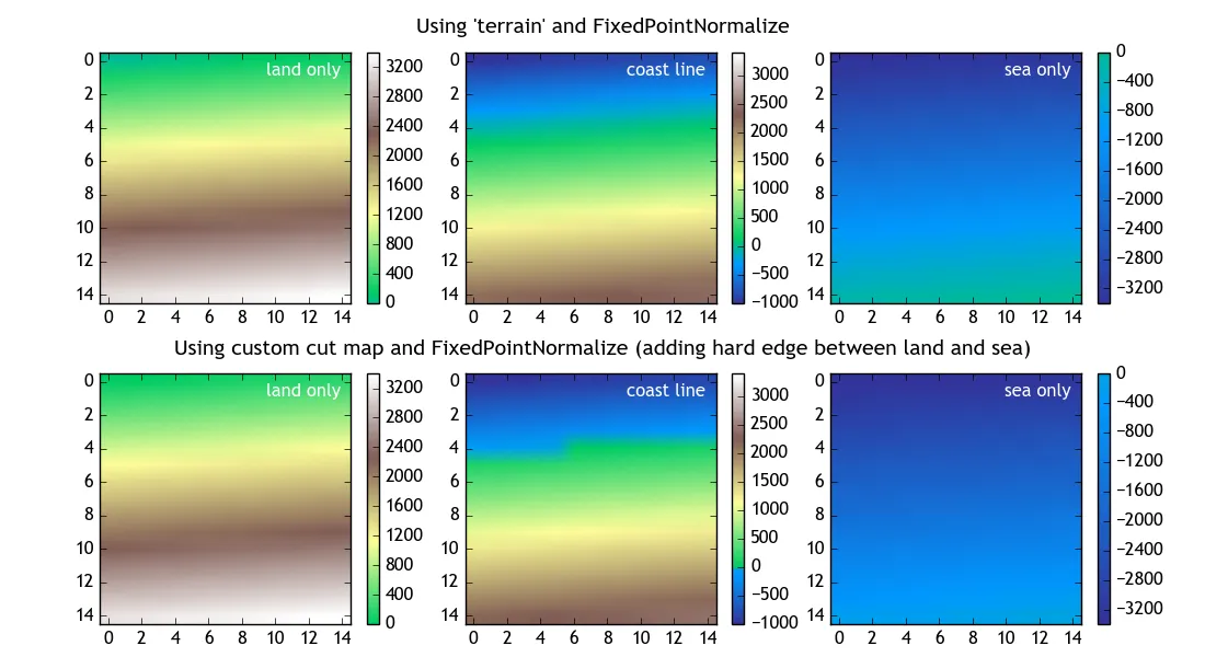
不幸的是，matplotlib没有提供类似Matlab中的demcmap功能。可能在Python basemap包中有一些内置功能，我不知道。

因此，我们可以在matplotlib自带选项中使用子类Normalize，构建围绕颜色图谱中间点的颜色规范化。这种技术可以在StackOverflow上的另一个问题中找到，并根据特定需求进行调整，即设置一个sealevel（可能最好选择为0）以及颜色图谱col_val（介于0和1之间）应与该海平面相对应的值。在地形图的情况下，看起来0.22，对应于蓝绿色，可能是一个不错的选择。
然后将Normalize实例作为imshow的参数给出。结果可以在下面的图片的第一行中看到。

由于海平面周围的平滑过渡，0附近的值呈现为蓝绿色，使得很难区分陆地和海洋。
因此，我们可以稍微改变地形图，并剪切掉那些颜色，从而更好地显示海岸线。这是通过组合介于0和0.17以及0.25到1之间的地图的两个部分来完成的，因此剪切了其中的一部分。

import numpy as np
import matplotlib.pyplot as plt
import matplotlib.colors

class FixPointNormalize(matplotlib.colors.Normalize):
    """ 
    Inspired by https://dev59.com/b2Ij5IYBdhLWcg3wilrB
    Subclassing Normalize to obtain a colormap with a fixpoint 
    somewhere in the middle of the colormap.

    This may be useful for a `terrain` map, to set the "sea level" 
    to a color in the blue/turquise range. 
    """
    def __init__(self, vmin=None, vmax=None, sealevel=0, col_val = 0.21875, clip=False):
        # sealevel is the fix point of the colormap (in data units)
        self.sealevel = sealevel
        # col_val is the color value in the range [0,1] that should represent the sealevel.
        self.col_val = col_val
        matplotlib.colors.Normalize.__init__(self, vmin, vmax, clip)

    def __call__(self, value, clip=None):
        x, y = [self.vmin, self.sealevel, self.vmax], [0, self.col_val, 1]
        return np.ma.masked_array(np.interp(value, x, y))

# Combine the lower and upper range of the terrain colormap with a gap in the middle
# to let the coastline appear more prominently.
# inspired by https://dev59.com/eV0Z5IYBdhLWcg3wzC5W
colors_undersea = plt.cm.terrain(np.linspace(0, 0.17, 56))
colors_land = plt.cm.terrain(np.linspace(0.25, 1, 200))
# combine them and build a new colormap
colors = np.vstack((colors_undersea, colors_land))
cut_terrain_map = matplotlib.colors.LinearSegmentedColormap.from_list('cut_terrain', colors)



# invent some data (height in meters relative to sea level)
data = np.linspace(-1000,2400,15**2).reshape((15,15))


# plot example data
fig, ax = plt.subplots(nrows = 2, ncols=3, figsize=(11,6) )
plt.subplots_adjust(left=0.08, right=0.95, bottom=0.05, top=0.92, hspace = 0.28, wspace = 0.15)

plt.figtext(.5, 0.95, "Using 'terrain' and FixedPointNormalize", ha="center", size=14)
norm = FixPointNormalize(sealevel=0, vmax=3400)
im = ax[0,0].imshow(data+1000, norm=norm, cmap=plt.cm.terrain)
fig.colorbar(im, ax=ax[0,0])

norm2 = FixPointNormalize(sealevel=0, vmax=3400)
im2 = ax[0,1].imshow(data, norm=norm2, cmap=plt.cm.terrain)
fig.colorbar(im2, ax=ax[0,1])

norm3 = FixPointNormalize(sealevel=0, vmax=0)
im3 = ax[0,2].imshow(data-2400.1, norm=norm3, cmap=plt.cm.terrain)
fig.colorbar(im3, ax=ax[0,2])

plt.figtext(.5, 0.46, "Using custom cut map and FixedPointNormalize (adding hard edge between land and sea)", ha="center", size=14)
norm4 = FixPointNormalize(sealevel=0, vmax=3400)
im4 = ax[1,0].imshow(data+1000, norm=norm4, cmap=cut_terrain_map)
fig.colorbar(im4, ax=ax[1,0])

norm5 = FixPointNormalize(sealevel=0, vmax=3400)
im5 = ax[1,1].imshow(data, norm=norm5, cmap=cut_terrain_map)
cbar = fig.colorbar(im5, ax=ax[1,1])

norm6 = FixPointNormalize(sealevel=0, vmax=0)
im6 = ax[1,2].imshow(data-2400.1, norm=norm6, cmap=cut_terrain_map)
fig.colorbar(im6, ax=ax[1,2])

for i, name in enumerate(["land only", "coast line", "sea only"]):
    for j in range(2):
        ax[j,i].text(0.96,0.96,name, ha="right", va="top", transform=ax[j,i].transAxes, color="w" )

plt.show()

- ImportanceOfBeingErnest