Python optimize.leastsq: 将圆适配到3D点集

Question

Python optimize.leastsq: 将圆适配到3D点集

pythonoptimizationcurve-fittingleast-squares

7

我正在尝试使用最小二乘圆拟合代码来处理3D数据集。我已经根据需要添加了z坐标来修改它以适应3D点。我的修改对于一个点集很好，但对于另一个点集效果很差。如果代码有错误，请查看一下。

import trig_items
import numpy as np
from trig_items import *
from numpy import *
from matplotlib import pyplot as p
from scipy import optimize

# Coordinates of the 3D points
##x = r_[36, 36, 19, 18, 33, 26]
##y = r_[14, 10, 28, 31, 18, 26]
##z = r_[0, 1, 2, 3, 4, 5]

x = r_[ 2144.18908574,  2144.26880854,  2144.05552972,  2143.90303742,  2143.62520676,
  2143.43628579,  2143.14005775,  2142.79919654,  2142.51436023,  2142.11240866,
  2141.68564346,  2141.29333828,  2140.92596405,  2140.3475612,   2139.90848046,
  2139.24661021,  2138.67384709,  2138.03313547,  2137.40301734,  2137.40908256,
  2137.06611224,  2136.50943781,  2136.0553113,   2135.50313189,  2135.07049922,
  2134.62098139,  2134.10459535,  2133.50838433,  2130.6600465,   2130.03537342,
  2130.04047644,  2128.83522468,  2127.79827542,  2126.43513385,  2125.36700593,
  2124.00350543,  2122.68564431,  2121.20709478,  2119.79047011,  2118.38417647,
  2116.90063343,  2115.52685778,  2113.82246629,  2112.21159431,  2110.63180117,
  2109.00713198,  2108.94434529,  2106.82777156,  2100.62343757,  2098.5090226,
  2096.28787738,  2093.91550703,  2091.66075061,  2089.15316429,  2086.69753869,
  2084.3002414,   2081.87590579,  2079.19141866,  2076.5394574,   2073.89128676,
  2071.18786213]
y = r_[ 725.74913818,  724.43874065,  723.15226506,  720.45950581,  717.77827954,
  715.07048092,  712.39633862,  709.73267688,  707.06039438,  704.43405908,
  701.80074596,  699.15371526,  696.5309022,   693.96109921,  691.35585501,
  688.83496327,  686.32148661,  683.80286662,  681.30705568,  681.30530975,
  679.66483676,  678.01922321,  676.32721779,  674.6667554,   672.9658024,
  671.23686095,  669.52021535,  667.84999077,  659.19757984,  657.46179949,
  657.45700508,  654.46901086,  651.38177517,  648.41739432,  645.32356976,
  642.39034578,  639.42628453,  636.51107198,  633.57732055,  630.63825133,
  627.75308356,  624.80162215,  622.01980232,  619.18814892,  616.37688894,
  613.57400131,  613.61535723,  610.4724493,   600.98277781,  597.84782844,
  594.75983001,  591.77946964,  588.74874068,  585.84525834,  582.92311166,
  579.99564481,  577.06666417,  574.30782762,  571.54115037,  568.79760614,
  566.08551098]
z = r_[ 339.77146775,  339.60021095,  339.47645894,  339.47130963,  339.37216218,
  339.4126132,   339.67942046,  339.40917728,  339.39500353,  339.15041461,
  339.38959195,  339.3358209,   339.47764895,  339.17854867,  339.14624071,
  339.16403926,  339.02308811,  339.27011082,  338.97684183,  338.95087698,
  338.97321177,  339.02175448,  339.02543922,  338.88725411,  339.06942374,
  339.0557553,   339.04414618,  338.89234303,  338.95572249,  339.00880416,
  339.00413073,  338.91080374,  338.98214758,  339.01135789,  338.96393537,
  338.73446188,  338.62784913,  338.72443217,  338.74880562,  338.69090173,
  338.50765186,  338.49056867,  338.57353355,  338.6196255,   338.43754399,
  338.27218569,  338.10587265,  338.43880881,  338.28962141,  338.14338705,
  338.25784154,  338.49792568,  338.15572139,  338.52967693,  338.4594245,
  338.1511823,   338.03711207,  338.19144663,  338.22022045,  338.29032321,
  337.8623197 ]

# coordinates of the barycenter
xm = mean(x)
ym = mean(y)
zm = mean(z)

### Basic usage of optimize.leastsq

def calc_R(xc, yc, zc):
    """ calculate the distance of each 3D points from the center (xc, yc, zc) """
    return sqrt((x - xc) ** 2 + (y - yc) ** 2 + (z - zc) ** 2)

def func(c):
    """ calculate the algebraic distance between the 3D points and the mean circle centered at c=(xc, yc, zc) """
    Ri = calc_R(*c)
    return Ri - Ri.mean()

center_estimate = xm, ym, zm
center, ier = optimize.leastsq(func, center_estimate)
##print center

xc, yc, zc = center
Ri       = calc_R(xc, yc, zc)
R        = Ri.mean()
residu   = sum((Ri - R)**2)
print 'R =', R

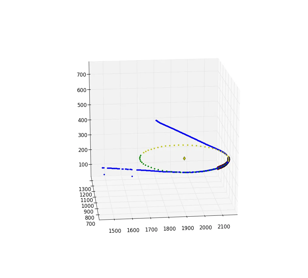
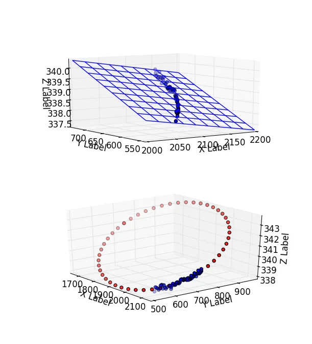
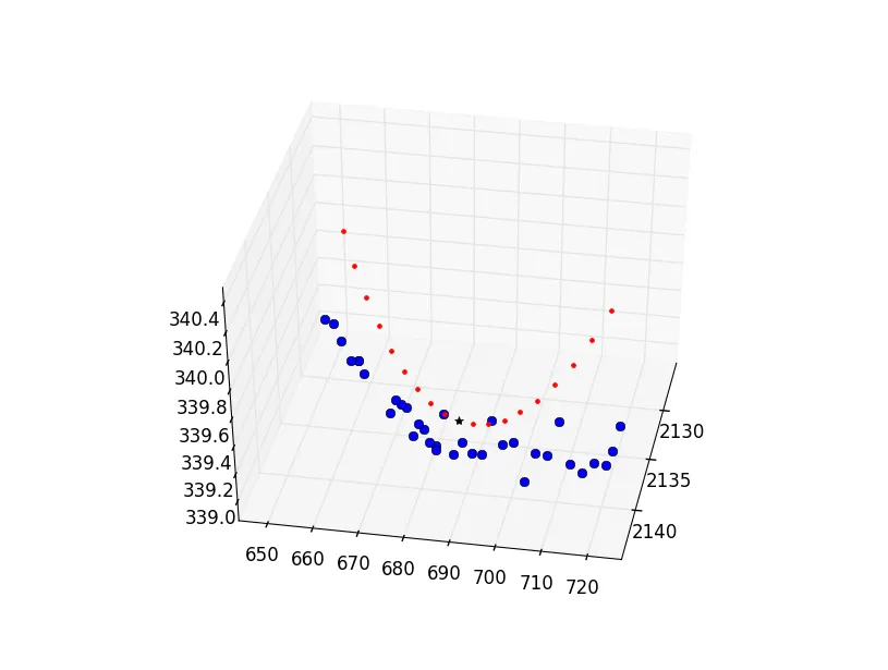
所以，对于第一组被注释的x, y, z（在代码中），它运行良好：输出结果为R = 39.0097846735。如果我使用第二组点运行代码（取消注释），则得到的半径为R = 108576.859834，几乎是直线。我绘制了最后一个。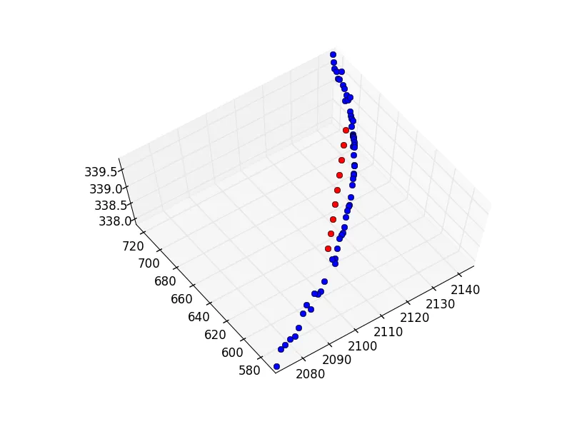

蓝色点是给定数据集，红色点是半径R = 108576.859834的弧。显然，给定的数据集比结果半径小得多。

这里是另一组点。

很明显，最小二乘法不能正确工作。

请帮忙解决这个问题。

更新：

这是我的解决方案：

### fit 3D arc into a set of 3D points             ###
### output is the centre and the radius of the arc ###
def fitArc3d(arr, eps = 0.0001):
    # Coordinates of the 3D points
    x = numpy.array([arr[k][0] for k in range(len(arr))])
    y = numpy.array([arr[k][4] for k in range(len(arr))])
    z = numpy.array([arr[k][5] for k in range(len(arr))])
    # coordinates of the barycenter
    xm = mean(x)
    ym = mean(y)
    zm = mean(z)
    ### gradient descent minimisation method ###
    pnts = [[x[k], y[k], z[k]] for k in range(len(x))]
    meanP = Point(xm, ym, zm) # mean point
    Ri = [Point(*meanP).distance(Point(*pnts[k])) for k in range(len(pnts))] # radii to the points
    Rm = math.fsum(Ri) / len(Ri) # mean radius
    dR = Rm + 10 # difference between mean radii
    alpha = 0.1
    c = meanP
    cArr = []
    while dR  > eps:
        cArr.append(c)
        Jx = math.fsum([2 * (x[k] - c[0]) * (Ri[k] - Rm) / Ri[k] for k in range(len(Ri))])
        Jy = math.fsum([2 * (y[k] - c[1]) * (Ri[k] - Rm) / Ri[k] for k in range(len(Ri))])
        Jz = math.fsum([2 * (z[k] - c[2]) * (Ri[k] - Rm) / Ri[k] for k in range(len(Ri))])
        gradJ = [Jx, Jy, Jz] # find gradient
        c = [c[k] + alpha * gradJ[k] for k in range(len(c)) if len(c) == len(gradJ)] # find new centre point
        Ri = [Point(*c).distance(Point(*pnts[k])) for k in range(len(pnts))] # calculate new radii
        RmOld = Rm
        Rm = math.fsum(Ri) / len(Ri) # calculate new mean radius
        dR = abs(Rm - RmOld) # new difference between mean radii

    return Point(*c), Rm

这段代码不是最优的（我没有时间进行精调），但它能够工作。

- user1329187

您可以在2D等效问题https://dev59.com/Wm7Xa4cB1Zd3GeqPpF8p#14835559中找到有用的解决方案。 - Hooked

如果你的数据通常看起来像这里的抛物线蓝点，平面拟合应该非常容易。因此，你可以轻松地将圆形拟合限制在2D版本中。（请参见我的更新。尽管你可能会使用不同的数据进行平面和圆形拟合） - mikuszefski

2个回答

0

感觉你在第一版代码中错过了一些约束条件。实现可以解释为将球拟合到3D点上。这就是为什么第二个数据列表的第二个半径几乎是一条直线。它的思考方式就像你给它一个大球上的小圆。

- Zack Yang

这应该作为注释而不是答案，会更好。 - Wasi Master

这并没有回答问题。一旦您拥有足够的声望，您将能够评论任何帖子；相反，提供不需要询问者澄清的答案。- 来自审核 - taylor.2317

网页内容由stack overflow 提供, 点击上面的

可以查看英文原文，
原文链接

- mikuszefski · Accepted Answer

我猜问题在于数据和相应的算法。如果最小二乘法产生一个局部抛物线最小值，那么简单的梯度方法就可以近似地朝向最小值方向。不幸的是，对于你的数据来说，这并不一定是真的。你可以通过保持一些xc和yc的粗略估计，并将平方残差的总和作为zc和R的函数进行绘制来检查这一点。我得到了一个回飞镖形的最小值。根据你的起始参数，你可能会停留在远离真正最小值的分支之一。一旦进入山谷，这可能非常平坦，以至于你超过了最大迭代次数或得到了在算法容差范围内被接受的东西。一如既往，起始参数越好，结果越好。不幸的是，你只有一个小圆弧，所以很难得到更好的结果。我不是Python专家，但我认为leastsq允许你玩弄雅可比矩阵和梯度方法。也尝试调整容差值。

简而言之：代码基本上看起来没问题，但你的数据是病态的，你必须适应这种数据的代码。

Karimäki有一个2D非迭代解决方案，也许你可以将这个方法改编为3D。你也可以查看这个。当然，你会找到更多的文献。

我刚刚使用Simplex算法检查了数据。如我所说，最小值表现不佳。在这里可以看到一些残差函数的截面。只有在xy平面上你才能得到一些合理的行为。zr和xr平面的特性使得寻找过程非常困难。

在一开始，单纯形算法找到了几个几乎稳定的解。在下面的图表中（蓝色x、紫色y、黄色z、绿色R），您可以看到它们是平坦的步骤。最后，该算法必须走过几乎平坦但非常拉伸的山谷，导致z和R的最终转化。然而，如果容差不足，我预计会有许多看起来像解决方案的区域。使用标准容差10^-5，算法在大约350次迭代后停止。我不得不将其设置为10^-10才能得到此解，即[1899.32，741.874，298.696，248.956]，这似乎相当不错。

更新

如早先提到的，解决方案取决于工作精度和所需精度。因此，您手动制作的梯度方法可能比内置的最小二乘拟合效果更好，因为这些值与之不同。尽管如此，这是我的版本，它进行了两步拟合。首先，我对数据拟合一个平面。在接下来的一步中，我在此平面内拟合一个圆。两个步骤都使用了最小二乘法。这一次它奏效了，因为每个步骤都避免了临界形状的极小值。（当弧段变得很小且数据几乎排在一条直线上时，平面拟合自然会遇到问题。但这将发生在所有算法中）。

from math import *
from matplotlib import pyplot as plt
from scipy import optimize
import numpy as np
from mpl_toolkits.mplot3d import Axes3D
import pprint as pp

dataTupel=zip(xs,ys,zs) #your data from above

# Fitting a plane first
# let the affine plane be defined by two vectors, 
# the zero point P0 and the plane normal n0
# a point p is member of the plane if (p-p0).n0 = 0 

def distanceToPlane(p0,n0,p):
    return np.dot(np.array(n0),np.array(p)-np.array(p0))    

def residualsPlane(parameters,dataPoint):
    px,py,pz,theta,phi = parameters
    nx,ny,nz =sin(theta)*cos(phi),sin(theta)*sin(phi),cos(theta)
    distances = [distanceToPlane([px,py,pz],[nx,ny,nz],[x,y,z]) for x,y,z in dataPoint]
    return distances

estimate = [1900, 700, 335,0,0] # px,py,pz and zeta, phi
#you may automize this by using the center of mass data
# note that the normal vector is given in polar coordinates
bestFitValues, ier = optimize.leastsq(residualsPlane, estimate, args=(dataTupel))
xF,yF,zF,tF,pF = bestFitValues

point  = [xF,yF,zF]
normal = [sin(tF)*cos(pF),sin(tF)*sin(pF),cos(tF)]

# Fitting a circle inside the plane
#creating two inplane vectors
sArr=np.cross(np.array([1,0,0]),np.array(normal))#assuming that normal not parallel x!
sArr=sArr/np.linalg.norm(sArr)
rArr=np.cross(sArr,np.array(normal))
rArr=rArr/np.linalg.norm(rArr)#should be normalized already, but anyhow


def residualsCircle(parameters,dataPoint):
    r,s,Ri = parameters
    planePointArr = s*sArr + r*rArr + np.array(point)
    distance = [ np.linalg.norm( planePointArr-np.array([x,y,z])) for x,y,z in dataPoint]
    res = [(Ri-dist) for dist in distance]
    return res

estimateCircle = [0, 0, 335] # px,py,pz and zeta, phi
bestCircleFitValues, ier = optimize.leastsq(residualsCircle, estimateCircle,args=(dataTupel))

rF,sF,RiF = bestCircleFitValues
print bestCircleFitValues

# Synthetic Data
centerPointArr=sF*sArr + rF*rArr + np.array(point)
synthetic=[list(centerPointArr+ RiF*cos(phi)*rArr+RiF*sin(phi)*sArr) for phi in np.linspace(0, 2*pi,50)]
[cxTupel,cyTupel,czTupel]=[ x for x in zip(*synthetic)]

### Plotting
d = -np.dot(np.array(point),np.array(normal))# dot product
# create x,y mesh
xx, yy = np.meshgrid(np.linspace(2000,2200,10), np.linspace(540,740,10))
# calculate corresponding z
# Note: does not work if normal vector is without z-component
z = (-normal[0]*xx - normal[1]*yy - d)/normal[2]

# plot the surface, data, and synthetic circle
fig = plt.figure()
ax = fig.add_subplot(211, projection='3d')
ax.scatter(xs, ys, zs, c='b', marker='o')
ax.plot_wireframe(xx,yy,z)
ax.set_xlabel('X Label')
ax.set_ylabel('Y Label')
ax.set_zlabel('Z Label')
bx = fig.add_subplot(212, projection='3d')
bx.scatter(xs, ys, zs, c='b', marker='o')
bx.scatter(cxTupel,cyTupel,czTupel, c='r', marker='o')
bx.set_xlabel('X Label')
bx.set_ylabel('Y Label')
bx.set_zlabel('Z Label')
plt.show()

半径为245。这与另一种方法得到的结果接近（249）。因此，在误差范围内，我得到了相同的结果。平面拟合和圆形逼近数据

绘制的结果看起来合理。希望能有所帮助。