更新于10/27:我已经在答案中提供了实现一致缩放的详细步骤。基本上,对于每个Graphics对象,您需要将所有填充/边距固定为0,并手动指定plotRange和imageSize,以使1)plotRange包括所有图形2)imageSize = scale * plotRange。
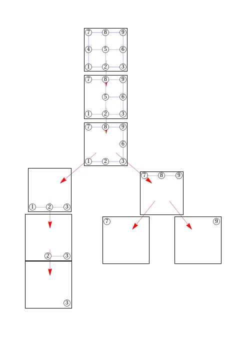
我在VertexRenderingFunction中使用"Inset"和"VertexCoordinates"来保证图形的子图之间具有一致的外观。这些子图被绘制成另一个图形的顶点,使用"Inset"。存在两个问题,一个是结果框未围绕图形进行裁剪(即,仍将具有一个顶点的图形放置在大框中),另一个是大小之间存在奇怪的变化(您可以看到一个框是垂直的)。有人能看到解决这些问题的方法吗?
这与早期的问题有关,即如何保持顶点大小相同,虽然Michael Pilat建议使用Inset可以使顶点以相同比例呈现,但整体比例可能不同。例如,在左分支上,由顶点2,3组成的图形相对于顶部图形中的“2,3”子图而言被拉伸了,即使我为两者都使用了绝对顶点定位。
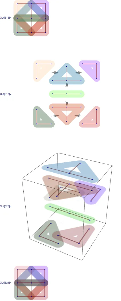
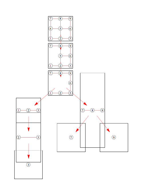
这是另一个示例,与之前的问题相同,但相对比例差异更加明显。目标是使第二张图片中的部分精确匹配第一张图片中的部分。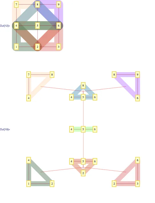
(来源:yaroslavvb.com)
任何其他关于图形操作美观可视化的建议都欢迎。
仍然不确定如何在完全泛化的情况下执行1),但给出了一个适用于由点和粗线(AbsoluteThickness)组成的Graphics的解决方案。
我在VertexRenderingFunction中使用"Inset"和"VertexCoordinates"来保证图形的子图之间具有一致的外观。这些子图被绘制成另一个图形的顶点,使用"Inset"。存在两个问题,一个是结果框未围绕图形进行裁剪(即,仍将具有一个顶点的图形放置在大框中),另一个是大小之间存在奇怪的变化(您可以看到一个框是垂直的)。有人能看到解决这些问题的方法吗?
这与早期的问题有关,即如何保持顶点大小相同,虽然Michael Pilat建议使用Inset可以使顶点以相同比例呈现,但整体比例可能不同。例如,在左分支上,由顶点2,3组成的图形相对于顶部图形中的“2,3”子图而言被拉伸了,即使我为两者都使用了绝对顶点定位。
(来源: yaroslavvb.com)
(*utilities*)intersect[a_, b_] := Select[a, MemberQ[b, #] &];
induced[s_] := Select[edges, #~intersect~s == # &];
Needs["GraphUtilities`"];
subgraphs[
verts_] := (gr =
Rule @@@ Select[edges, (Intersection[#, verts] == #) &];
Sort /@ WeakComponents[gr~Join~(# -> # & /@ verts)]);
(*graph*)
gname = {"Grid", {3, 3}};
edges = GraphData[gname, "EdgeIndices"];
nodes = Union[Flatten[edges]];
AppendTo[edges, #] & /@ ({#, #} & /@ nodes);
vcoords = Thread[nodes -> GraphData[gname, "VertexCoordinates"]];
(*decompose*)
edgesOuter = {};
pr[_, _, {}] := None;
pr[root_, elim_,
remain_] := (If[root != {}, AppendTo[edgesOuter, root -> remain]];
pr[remain, intersect[Rest[elim], #], #] & /@
subgraphs[Complement[remain, {First[elim]}]];);
pr[{}, {4, 5, 6, 1, 8, 2, 3, 7, 9}, nodes];
(*visualize*)
vrfInner =
Inset[Graphics[{White, EdgeForm[Black], Disk[{0, 0}, .05], Black,
Text[#2, {0, 0}]}, ImageSize -> 15], #] &;
vrfOuter =
Inset[GraphPlot[Rule @@@ induced[#2],
VertexRenderingFunction -> vrfInner,
VertexCoordinateRules -> vcoords, SelfLoopStyle -> None,
Frame -> True, ImageSize -> 100], #] &;
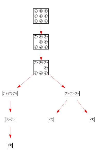
TreePlot[edgesOuter, Automatic, nodes,
EdgeRenderingFunction -> ({Red, Arrow[#1, 0.2]} &),
VertexRenderingFunction -> vrfOuter, ImageSize -> 500]
这是另一个示例,与之前的问题相同,但相对比例差异更加明显。目标是使第二张图片中的部分精确匹配第一张图片中的部分。
(来源:yaroslavvb.com)
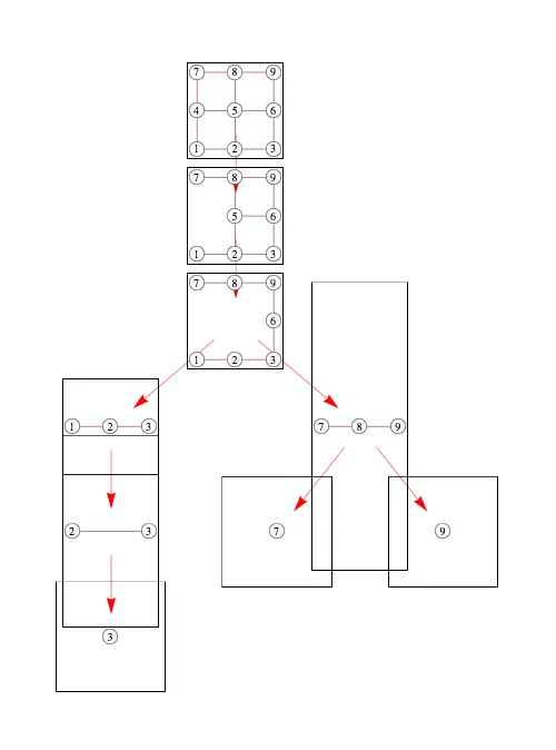
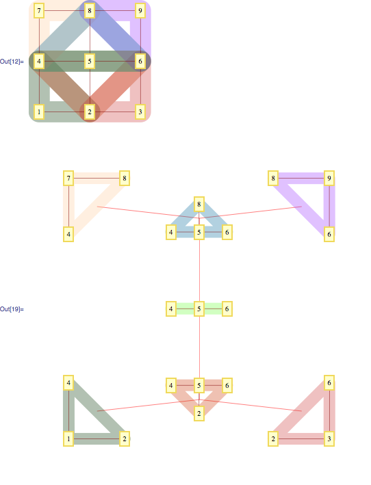
(* Visualize tree decomposition of a 3x3 grid *)

inducedGraph[set_] := Select[edges, # \[Subset] set &];
Subset[a_, b_] := (a \[Intersection] b == a);
graphName = {"Grid", {3, 3}};
edges = GraphData[graphName, "EdgeIndices"];
vars = Range[GraphData[graphName, "VertexCount"]];
vcoords = Thread[vars -> GraphData[graphName, "VertexCoordinates"]];

plotHighlight[verts_, color_] := Module[{vpos, coords},
   vpos =
    Position[Range[GraphData[graphName, "VertexCount"]],
     Alternatives @@ verts];
   coords = Extract[GraphData[graphName, "VertexCoordinates"], vpos];
   If[coords != {}, AppendTo[coords, First[coords] + .002]];
   Graphics[{color, CapForm["Round"], JoinForm["Round"],
     Thickness[.2], Opacity[.3], Line[coords]}]];

jedges = {{{1, 2, 4}, {2, 4, 5, 6}}, {{2, 3, 6}, {2, 4, 5, 6}}, {{4,
     5, 6}, {2, 4, 5, 6}}, {{4, 5, 6}, {4, 5, 6, 8}}, {{4, 7, 8}, {4,
     5, 6, 8}}, {{6, 8, 9}, {4, 5, 6, 8}}};
jnodes = Union[Flatten[jedges, 1]];

SeedRandom[1]; colors =
 RandomChoice[ColorData["WebSafe", "ColorList"], Length[jnodes]];
bags = MapIndexed[plotHighlight[#, bc[#] = colors[[First[#2]]]] &,
   jnodes];
Show[bags~
  Join~{GraphPlot[Rule @@@ edges, VertexCoordinateRules -> vcoords,
    VertexLabeling -> True]}, ImageSize -> Small]

bagCentroid[bag_] := Mean[bag /. vcoords];
findExtremeBag[vec_] := (
   vertList = First /@ vcoords;
   coordList = Last /@ vcoords;
   extremePos =
    First[Ordering[jnodes, 1,
      bagCentroid[#1].vec > bagCentroid[#2].vec &]];
   jnodes[[extremePos]]
   );

extremeDirs = {{1, 1}, {1, -1}, {-1, 1}, {-1, -1}};
extremeBags = findExtremeBag /@ extremeDirs;
extremePoses = bagCentroid /@ extremeBags;
vrfOuter =
  Inset[Show[plotHighlight[#2, bc[#2]],
     GraphPlot[Rule @@@ inducedGraph[#2],
      VertexCoordinateRules -> vcoords, SelfLoopStyle -> None,
      VertexLabeling -> True], ImageSize -> 100], #] &;

GraphPlot[Rule @@@ jedges, VertexRenderingFunction -> vrfOuter,
 EdgeRenderingFunction -> ({Red, Arrowheads[0], Arrow[#1, 0]} &),
 ImageSize -> 500,
 VertexCoordinateRules -> Thread[Thread[extremeBags -> extremePoses]]]
任何其他关于图形操作美观可视化的建议都欢迎。
intersection是因为Intersection会对列表进行排序。 - Yaroslav Bulatov