使用raster包进行空间自相关性分析

Question

亲爱的众人

问题

我尝试使用nfc、pgirmess、SpatialPack和spdep包计算空间自相关图。然而，我在定义距离的起点和终点时遇到了困难。我只对小距离下的空间自相关性感兴趣，但是这里要使用更小的区间。此外，由于栅格数据集相当大（1.8百万像素），使用这些包但SpatialPack会遇到内存问题。

因此，我尝试自己编写代码，使用raster包中的Moran函数。但是我的结果与其他包的结果有些不同，这可能是因为我的代码中有错误。如果我的代码没有错误，它至少可以帮助其他遇到类似问题的人。

问题

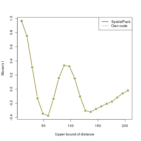
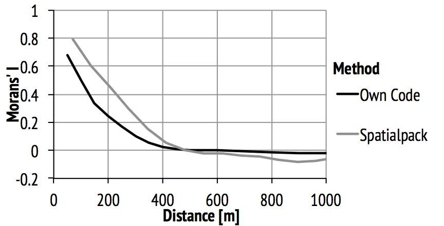
我不确定我的聚焦矩阵是否有误。请问中心像素是否需要被纳入？使用测试数据，我无法展示这些方法之间的差异，但在我的完整数据集上，存在差异，如下面的图片所示。但是，这些区间不完全相同（50m vs. 69m），因此这可能解释了部分差异。但是，在第一个区间，这种解释对我来说似乎不太合理。或者，我的栅格数据集的不规则形状和处理NA的不同方式会引起差异吗？

自己的方法与SpatialPack的比较

可运行示例

测试数据

计算测试数据的代码取自http://www.petrkeil.com/?p=1050#comment-416317

# packages used for the data generation
library(raster)
library(vegan) # will be used for PCNM

# empty matrix and spatial coordinates of its cells
side=30
my.mat <- matrix(NA, nrow=side, ncol=side)
x.coord <- rep(1:side, each=side)*5
y.coord <- rep(1:side, times=side)*5
xy <- data.frame(x.coord, y.coord)

# all paiwise euclidean distances between the cells
xy.dist <- dist(xy)

# PCNM axes of the dist. matrix (from 'vegan' package)
pcnm.axes <- pcnm(xy.dist)$vectors

# using 8th PCNM axis as my atificial z variable
z.value <- pcnm.axes[,8]*200 + rnorm(side*side, 0, 1)

# plotting the artificial spatial data
r <- rasterFromXYZ(xyz = cbind(xy,z.value))
plot(r, axes=F)

自己的代码

library(raster)
sp.Corr <- matrix(nrow = 0,ncol = 2)
formerBreak <- 0 #for the first run important
for (i in c(seq(10,200,10))) #Calculate the Morans I for these bins
{
  cat(paste0("..",i)) #print the bin, which is currently calculated
  w = focalWeight(r,d = i,type = 'circle')
  wTemp <- w #temporarily saves the weigtht matrix
  if (formerBreak>0) #if it is the second run
  {
    midpoint <- ceiling(ncol(w)/2) # get the midpoint      
    w[(midpoint-formerBreak):(midpoint+formerBreak),(midpoint-formerBreak):(midpoint+formerBreak)] <- w[(midpoint-formerBreak):(midpoint+formerBreak),(midpoint-formerBreak):(midpoint+formerBreak)]*(wOld==0)#set the previous focal weights to 0
    w <- w*(1/sum(w)) #normalizes the vector to sum the weights to 1
  }
  wOld <- wTemp #save this weight matrix for the next run
  mor <- Moran(r,w = w)
  sp.Corr <- rbind(sp.Corr,c(Moran =mor,Distance = i))
  formerBreak <- i/res(r)[1]#divides the breaks by the resolution of the raster to be able to translate them to the focal window
}
plot(x=sp.Corr[,2],y = sp.Corr[,1],type = "l",ylab = "Moran's I",xlab="Upper bound of distance")

计算空间相关图的其他方法

library(SpatialPack)
sp.Corr <- summary(modified.ttest(z.value,z.value,coords = xy,nclass = 21))
plot(x=sp.Corr$coef[,1],y = data$coef[,4],type = "l",ylab = "Moran's I",xlab="Upper bound of distance")

library(ncf)
ncf.cor <- correlog(x.coord, y.coord, z.value,increment=10, resamp=1)
plot(ncf.cor)

- Benasso

---

你能告诉我们更多关于你使用的数据吗？你发现了什么差异？特别是，它们是否处于球面坐标（经度/纬度）而不是平面坐标系中？这可能是差异的一个可能原因，因为raster::focalWeight考虑到了这一点，但我认为SpatialPack::modified.ttest没有考虑到（它似乎假设平面坐标系）。 - Robert Hijmans

它们都不是在球坐标系中。它们都是在瑞士国家网格中投影的。 - Benasso

Answer 1

为了比较相关图的结果，在您的情况下，需要考虑两件事。 (i) 您的代码仅适用于与您的栅格分辨率成比例的bin。在这种情况下，bin中的一点差异可能会包括或排除重要数量的对。 (ii) 栅格的不规则形状对于计算某个距离间隔的相关性所考虑的对有很强的影响。因此，您的代码应处理这两个问题，允许任何bin长度的值，并考虑栅格的不规则形状。以下是修改您的代码以解决这些问题的方法。

# SpatialPack correlation
library(SpatialPack)
test <- modified.ttest(z.value,z.value,coords = xy,nclass = 21)

# Own correlation
bins <- test$upper.bounds
library(raster)
sp.Corr <- matrix(nrow = 0,ncol = 2)
for (i in bins) {
  cat(paste0("..",i)) #print the bin, which is currently calculated
  w = focalWeight(r,d = i,type = 'circle')
  wTemp <- w #temporarily saves the weigtht matrix
  if (i > bins[1]) {
    midpoint <- ceiling(dim(w)/2) # get the midpoint      
    half_range <- floor(dim(wOld)/2)
    w[(midpoint[1] - half_range[1]):(midpoint[1] + half_range[1]),
      (midpoint[2] - half_range[2]):(midpoint[2] + half_range[2])] <- 
        w[(midpoint[1] - half_range[1]):(midpoint[1] + half_range[1]),
      (midpoint[2] - half_range[2]):(midpoint[2] + half_range[2])]*(wOld==0)
    w <- w * (1/sum(w)) #normalizes the vector to sum the weights to 1
  }
  wOld <- wTemp #save this weight matrix for the next run
  mor <- Moran(r,w=w)
  sp.Corr <- rbind(sp.Corr,c(Moran =mor,Distance = i))
}
# Comparing
plot(x=test$upper.bounds, test$imoran[,1], col = 2,type = "b",ylab = "Moran's I",xlab="Upper bound of distance", lwd = 2)
lines(x=sp.Corr[,2],y = sp.Corr[,1], col = 3)
points(x=sp.Corr[,2],y = sp.Corr[,1], col = 3)
legend('topright', legend = c('SpatialPack', 'Own code'), col = 2:3, lty = 1, lwd = 2:1)

图像显示使用SpatialPack包和自己的代码得到的结果相同。

- Erick Chacon