Scikit-image扩展主动轮廓(蛇)

11
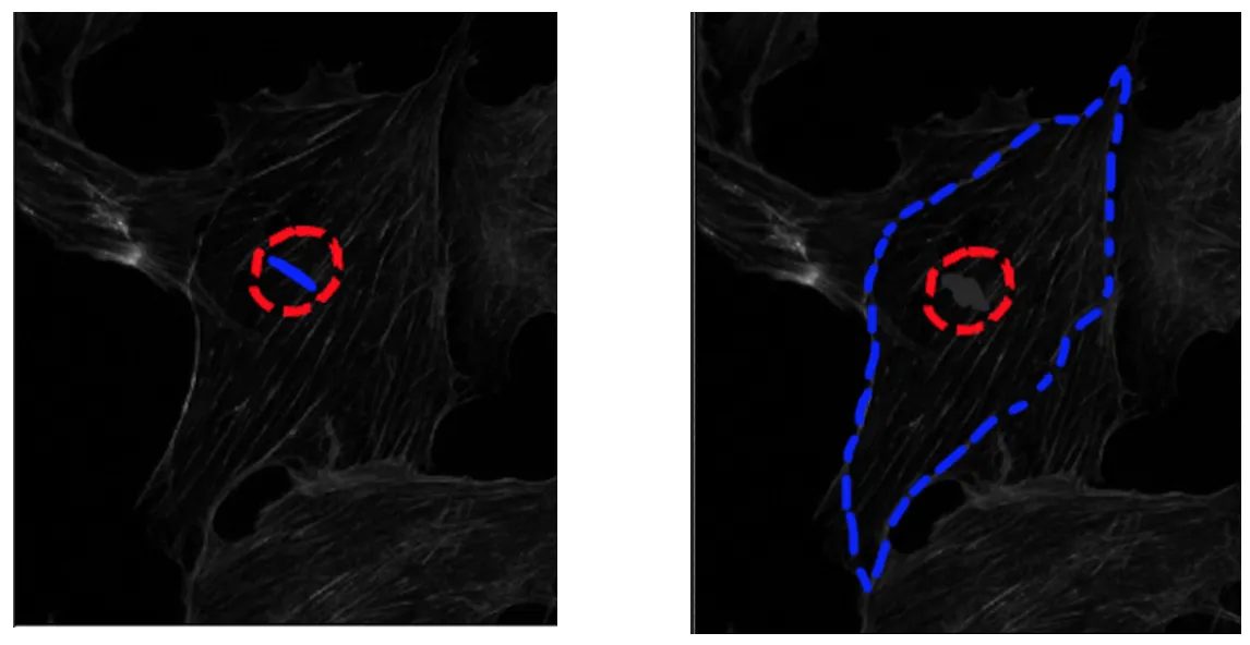
我按照这个链接的示例进行了操作。然而,轮廓从初始点开始收缩。是否可能做出扩张的轮廓?我想要像图片所示的那样。左边的图片是它的样子,右边的图片是我想要的样子 - 扩张而不是收缩。红色圆圈是起始点,蓝色轮廓是经过n次迭代后的结果。是否有一个参数可以设置 - 我查看了所有参数,但似乎没有设置这个的。此外,当提到“主动轮廓”时,通常是否假定轮廓会收缩?我阅读了这篇论文并认为它既可以收缩也可以扩张。
img = data.astronaut()
img = rgb2gray(img)

s = np.linspace(0, 2*np.pi, 400)
x = 220 + 100*np.cos(s)
y = 100 + 100*np.sin(s)
init = np.array([x, y]).T

if not new_scipy:
    print('You are using an old version of scipy. '
          'Active contours is implemented for scipy versions '
          '0.14.0 and above.')

if new_scipy:
    snake = active_contour(gaussian(img, 3),
                           init, alpha=0.015, beta=10, gamma=0.001)

    fig = plt.figure(figsize=(7, 7))
    ax = fig.add_subplot(111)
    plt.gray()
    ax.imshow(img)
    ax.plot(init[:, 0], init[:, 1], '--r', lw=3)
    ax.plot(snake[:, 0], snake[:, 1], '-b', lw=3)
    ax.set_xticks([]), ax.set_yticks([])
    ax.axis([0, img.shape[1], img.shape[0], 0])
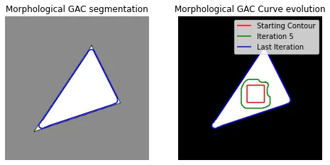
enter image description here


你可以尝试将 max_px_move 设置为 -1,但我不知道那是否有效。 - Stefan van der Walt
你找到了一种方法来做这件事吗? - ViktoriaDoneva
1个回答

8
你需要的是将“气球力”添加到蛇中。
蛇算法被定义为最小化3个能量 - 连续性、曲率和梯度,分别对应于代码中的alpha、beta和gamma。前两个(合称内部能量)在点(在曲线上)被拉得越来越近时得到最小化,即收缩。如果它们扩张,则能量增加,这是蛇算法不允许的。
但是,这个最初的算法在1987年提出时存在一些问题。其中一个问题是,在平坦区域(梯度为零的地方),算法无法收敛,什么也做不了。已经提出了几种修改方法来解决这个问题。这里感兴趣的解决方案是LD Cohen在1989年提出的“气球力”。
气球力指导轮廓在图像的非信息区域中,即图像的梯度太小,无法将轮廓推向边界的区域。负值会收缩轮廓,而正值会扩展轮廓。将其设置为零将禁用气球力。
另一个改进是形态蛇,它使用形态学运算符(如膨胀或腐蚀)在二进制数组上,而不是在浮点数数组上解决PDE,这是主动轮廓的标准方法。这使得形态蛇比传统的对应物更快,数值上更加稳定。

Scikit-image使用上述两个改进的实现是morphological_geodesic_active_contour。它有一个参数balloon

在没有任何真实原始图像的情况下,让我们创建一个玩具图像并处理它:

import numpy as np
import matplotlib.pyplot as plt
from skimage.segmentation import morphological_geodesic_active_contour, inverse_gaussian_gradient
from skimage.color import rgb2gray
from skimage.util import img_as_float
from PIL import Image, ImageDraw
   
im = Image.new('RGB', (250, 250), (128, 128, 128))
draw = ImageDraw.Draw(im)
draw.polygon(((50, 200), (200, 150), (150, 50)), fill=(255, 255, 0), outline=(0, 0, 0))
im = np.array(im)
im = rgb2gray(im)
im = img_as_float(im)
plt.imshow(im, cmap='gray')

这给我们下面的图片。

enter image description here

现在让我们创建一个函数,它将帮助我们存储迭代结果:
def store_evolution_in(lst):
    """Returns a callback function to store the evolution of the level sets in
    the given list.
    """

    def _store(x):
        lst.append(np.copy(x))

    return _store

这种方法需要对图像进行预处理以突出轮廓。可以使用函数inverse_gaussian_gradient来完成此操作,尽管用户可能想定义自己的版本。 MorphGAC分割的质量在很大程度上取决于这个预处理步骤。
gimage = inverse_gaussian_gradient(im)

以下是我们的起点 - 一个正方形。

init_ls = np.zeros(im.shape, dtype=np.int8)
init_ls[120:-100, 120:-100] = 1

绘制演变过程的中间结果列表
evolution = []
callback = store_evolution_in(evolution)

现在,morphological_geodesic_active_contour需要以下魔术行来实现气球膨胀:

ls = morphological_geodesic_active_contour(gimage, 50, init_ls, 
                                           smoothing=1, balloon=1,
                                            threshold=0.7,
                                           iter_callback=callback)

现在让我们绘制结果:
fig, axes = plt.subplots(1, 2, figsize=(8, 8))
ax = axes.flatten()

ax[0].imshow(im, cmap="gray")
ax[0].set_axis_off()
ax[0].contour(ls, [0.5], colors='b')
ax[0].set_title("Morphological GAC segmentation", fontsize=12)

ax[1].imshow(ls, cmap="gray")
ax[1].set_axis_off()
contour = ax[1].contour(evolution[0], [0.5], colors='r')
contour.collections[0].set_label("Starting Contour")
contour = ax[1].contour(evolution[5], [0.5], colors='g')
contour.collections[0].set_label("Iteration 5")
contour = ax[1].contour(evolution[-1], [0.5], colors='b')
contour.collections[0].set_label("Last Iteration")
ax[1].legend(loc="upper right")
title = "Morphological GAC Curve evolution"
ax[1].set_title(title, fontsize=12)

plt.show()

enter image description here

红色正方形是我们的起点(初始轮廓),蓝色轮廓来自最终迭代。

网页内容由stack overflow 提供, 点击上面的
可以查看英文原文,
原文链接