ggplot2中坐标轴文本的上标

Question

我希望使用ggplot2创建一个图表，其中坐标轴上有上标，而不是显示未格式化的数字。我知道有许多答案可以更改轴标签，但不能更改轴文本。我不是想更改图表的标签，而是更改轴上的文本。

示例：

x<-c('2^-5','2^-3','2^-1','2^1','2^2','2^3','2^5','2^7','2^9','2^11','2^13')
y<-c('2^-5','2^-3','2^-1','2^1','2^2','2^3','2^5','2^7','2^9','2^11','2^13')
df<-data.frame(x,y)
p<-ggplot()+
  geom_point(data=df,aes(x=x,y=y),size=4)
p

我希望x轴显示相同的数字，但不要有箭头。

- Jack Armstrong

---

请修改以下内容：https://dev59.com/QFoU5IYBdhLWcg3w7qMt?rq=1。 - NelsonGon

这不是重复的标签，这是轴文字。 - Jack Armstrong

是的，我设计它们就是因为如果它是数字，那么你会像绘制任何其他图表一样绘制数字，我想将它们保留为字符，但你也可以有因子。 - Jack Armstrong

那么，您想评估与轴上的文本相等的数字还是仅删除插入符号？ - NelsonGon

删除插入符号。 - Jack Armstrong

Answer 1

编辑： 仅使用base方法：

df %>% 
  mutate_all(as.character)->new_df
res<-unlist(Map(function(x) eval(parse(text=x)),new_df$x))#replace with y for y
to_use<-unlist(lapply(res,as.expression))
split_text<-strsplit(gsub("\\^"," ",names(to_use))," ")
join_1<-as.numeric(sapply(split_text,"[[",1)) #tidyr::separate might help, less robust for numeric(I think)
join_2<-as.numeric(sapply(split_text,"[[",2))
to_use_1<-sapply(seq_along(join_1),function(x) parse(text=paste(join_1[x],"^",
                                                join_2[x])))

上述步骤可以简化为更少的步骤，我发布了我所采取的逐步方法。仅针对x的结果，同样的操作可以用于y。

new_df %>%   
ggplot()+
  geom_point(aes(x=x,y=y),size=4)+
 scale_x_discrete(breaks=df$x,labels=to_use_1)#replace with y and scale_y_discrete for y

情节：

原始错误答案：

我没有遵循标准的tidyverse实践，而是使用了$，你可以将其替换为.，虽然在这种情况下它并不重要，因为重点在于标签。

    library(dplyr)
   df %>% 
          mutate(new_x=gsub("\\^"," ",x),
                 new_y=gsub("\\^"," ",y))->new_df
        new_df %>%   
        ggplot()+
          geom_point(aes(x=x,y=y),size=4)+
         scale_x_discrete(breaks=x,labels=new_df$new_x)+
          scale_y_discrete(breaks=y,labels=new_df$new_y)

- NelsonGon

---

我认为这是一个不错的开始，但现在数字顺序错了。 - Jack Armstrong

不好意思，请问您能详细说明一下吗？ - NelsonGon

例如，2的11次方比2的3次方小。 - Jack Armstrong

不确定为什么我们有不同的结果。你是使用问题中的数据还是其他数据？我已经几天没看这个了，可能需要看看你正在使用的代码和/或数据。 - NelsonGon

Answer 2

这可以通过在GitHub软件包中找到的scale_x_log2和scale_y_log2函数来完成。

首先，安装该软件包。

devtools::install_github("jrnold/rubbish")

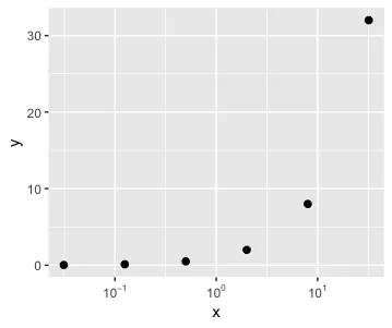
然后，将变量强制转换为数值型。我会使用原始数据框的副本进行操作。

df1 <- df
df1[] <- lapply(df1, function(x){
  x <- as.character(x)
  sapply(x, function(.x)eval(parse(text = .x)))
})

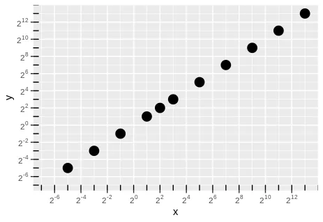
现在，将其绘制成图表。

library(jrnoldmisc)
library(ggplot2)
library(MASS)
library(scales)

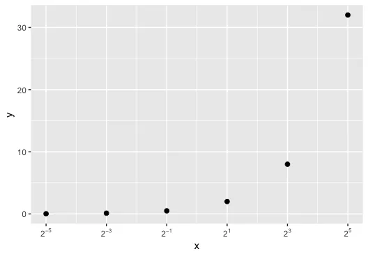
a <- ggplot(df1, aes(x = x, y = y, size = 4)) + 
  geom_point(show.legend = FALSE) +
  scale_x_log2(limits = c(0.01, NA), 
                labels = trans_format("log2", math_format(2^.x)),
                breaks = trans_breaks("log2", function(x) 2^x, n = 10)) +
  scale_y_log2(limits = c(0.01, NA),
                labels = trans_format("log2", math_format(2^.x)),
                breaks = trans_breaks("log2", function(x) 2^x, n = 10))
a + annotation_logticks(base = 2)

中译英：

编辑。

根据评论中的讨论，以下是另外两种给出不同轴标签的方法。

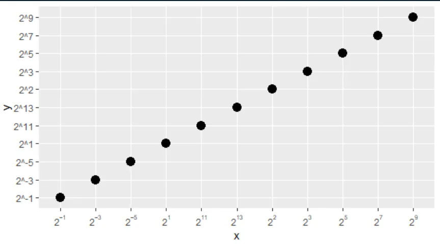
1. 每个刻度标记都有轴标签。设置limits = c(1.01, NA)和函数参数n = 11，一个奇数。
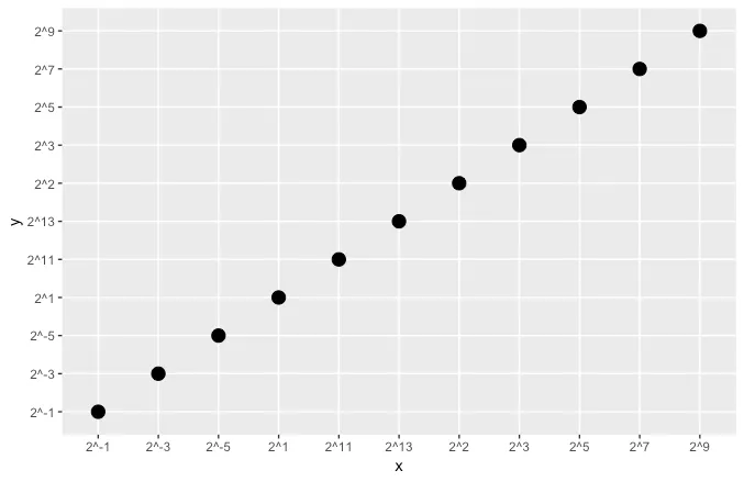
2. 轴标签在奇数指数上。保持limits = c(0.01, NA)，更改为function(x) 2^(x - 1), n = 11。

只有说明，没有图表。

第一种方法。

a <- ggplot(df1, aes(x = x, y = y, size = 4)) + 
  geom_point(show.legend = FALSE) +
  scale_x_log2(limits = c(1.01, NA), 
                labels = trans_format("log2", math_format(2^.x)),
                breaks = trans_breaks("log2", function(x) 2^(x), n = 11)) +
  scale_y_log2(limits = c(1.01, NA),
                labels = trans_format("log2", math_format(2^.x)),
                breaks = trans_breaks("log2", function(x) 2^(x), n = 11))
a + annotation_logticks(base = 2)

第二个。

a <- ggplot(df1, aes(x = x, y = y, size = 4)) + 
  geom_point(show.legend = FALSE) +
  scale_x_log2(limits = c(0.01, NA), 
               labels = trans_format("log2", math_format(2^.x)),
               breaks = trans_breaks("log2", function(x) 2^(x - 1), n = 11)) +
  scale_y_log2(limits = c(0.01, NA),
               labels = trans_format("log2", math_format(2^.x)),
               breaks = trans_breaks("log2", function(x) 2^(x - 1), n = 11))
a + annotation_logticks(base = 2)

- Rui Barradas

---

是否可以在奇数上或每个刻度线上放置刻度标记，而不仅仅是偶数上的？ - Jack Armstrong

@JackArmstrong 是的，我刚刚在sclae_*_log2调用中测试了limits = c(1.01, NA)，现在它会在每个刻度线上打印。 - Rui Barradas

不使用限制，而是在断点内使用 = trans_breaks("log2", function(x) 2^(x-1), n = 10))。 - Jack Armstrong

@JackArmstrong 你说得完全正确，我没有想到那一点。但是它只会在奇数指数上给出标签，而使用 limits 则会在每个刻度上都给出标签。 - Rui Barradas

@JackArmstrong 好的，我知道了。我把 function(x) 2^(x), n = 11 中的参数 n 改成了奇数。再加上 limits = c(1.01, NA) 就能在每个刻度上显示标签了。我需要编辑答案吗？ - Rui Barradas

如果你想用其他可能的方式，当然可以。我认为不需要图片。人们应该能够阅读。 - Jack Armstrong

Answer 3

你可以向scale_x_***和scale_y_***函数的labels参数提供一个功能，以生成带有上标（或其他格式）的标签。请参见下面的示例。原始答案可以翻译为"最初的回答"。

library(jrnoldmisc)
library(ggplot2)

df<-data.frame(x=2^seq(-5,5,2),
               y=2^seq(-5,5,2))

ggplot(df) +
  geom_point(aes(x=x,y=y),size=2)  +
  scale_x_log2(breaks=2^seq(-5,5,2),
               labels=function(x) parse(text=paste("2^",round(log2(x),2))))

ggplot(df) +
  geom_point(aes(x=x,y=y),size=2)  +
  scale_x_continuous(breaks=c(2^-5, 2^seq(1,5,2)),
                     labels=function(x) parse(text=paste("2^",round(log2(x),2))))

ggplot(df) +
  geom_point(aes(x=x,y=y),size=2)  +
  scale_x_log10(breaks=10^seq(-1,1,1),
                labels=function(x) parse(text=paste("10^",round(log10(x),2))))

- eipi10