R提供Lloyd's算法作为kmeans()的一个选项;默认算法由Hartigan和Wong(1979)提出,更加聪明。像MacQueen的算法(MacQueen,1967)一样,它在任何时候移动一个点时更新质心;它还在检查最接近的簇时做了聪明的(节省时间的)选择。然而,Lloyd的k-means算法是所有这些聚类算法中最简单的。
Lloyd算法(Lloyd,1957)将一组观察值或案例(想象成nxp矩阵的行或Reals中的点)聚类成个组。它试图最小化簇内平方和
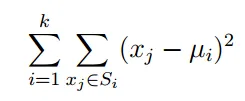
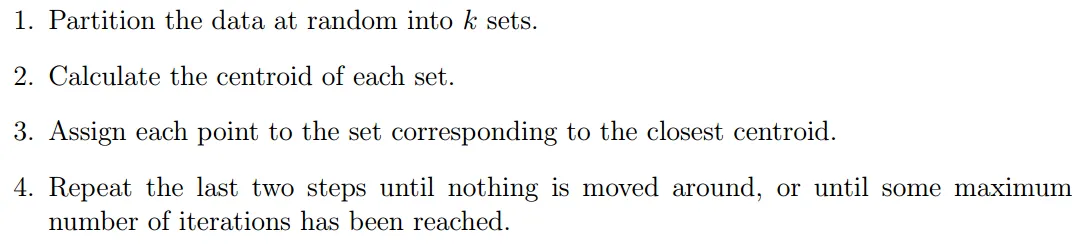
其中u_i是簇S_i中所有点的平均值。该算法的步骤如下(我会省略详细说明的形式):
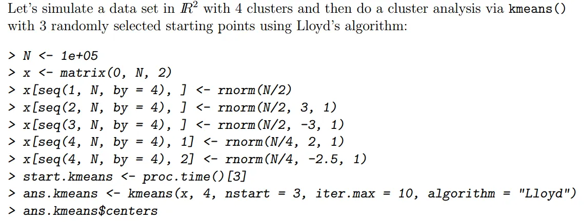
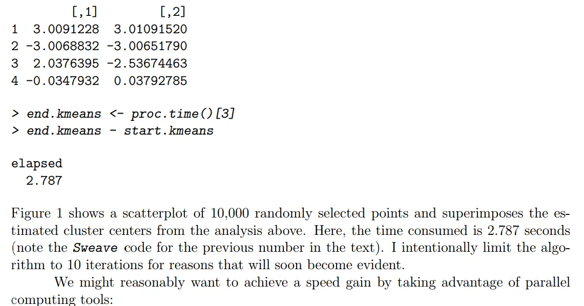
然而,在考虑多个起始点时,R的实现存在问题。我应该指出,通常考虑几个不同的起始点比较谨慎,因为算法保证收敛,但不能保证收敛到全局最优解。这对于大型、高维度问题尤其如此。我将从一个简单的例子(大型、不特别困难)开始。
(这里我将粘贴一些图片,因为我们无法使用latex编写数学公式)
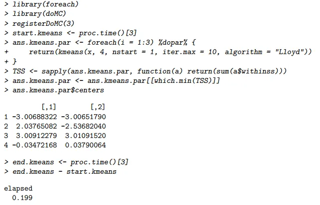
请注意,该解决方案与早期实现的解决方案非常相似,尽管簇的排序是任意的。更重要的是,该任务仅花费了0.199秒并行执行!当然,这听起来太好以至于不可思议:使用3个处理器核心应该在最佳情况下只需要第一次(顺序)运行时间的三分之一。这是一个问题吗?听起来像是免费午餐。偶尔享受免费午餐没有问题,对吧?
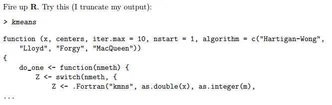
这并不总是适用于R函数,但有时我们有机会直接查看代码。这就是其中之一。我将把此代码放入文件mykmeans.R中,并手动编辑它,在各个位置插入cat()语句。下面是一种聪明的方法,使用sink()(尽管这在Sweave中似乎不起作用,但可以交互式地使用):
> sink("mykmeans.R")
> kmeans
> sink()
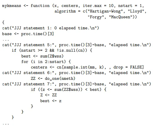
现在正在编辑文件,更改函数名称并添加cat()语句。请注意,您还必须删除一个结尾行:
然后,我们可以使用mykmeans()来重复我们的探索:
> source("mykmeans.R")
> start.kmeans <- proc.time()[3]
> ans.kmeans <- mykmeans(x, 4, nstart = 3, iter.max = 10, algorithm = "Lloyd")
JJJ statement 1: 0 elapsed time.
JJJ statement 5: 2.424 elapsed time.
JJJ statement 6: 2.425 elapsed time.
JJJ statement 7: 2.52 elapsed time.
JJJ statement 6: 2.52 elapsed time.
JJJ statement 7: 2.563 elapsed time.
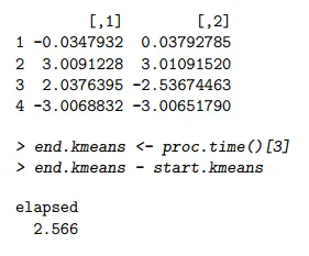
现在我们可以开始了:大部分时间都用在语句5之前了(当然我知道这点,这就是为什么语句5是5而不是2)...你可以继续玩耍它。
以下是代码:
N <- 100000
x <- matrix(0, N, 2)
x[seq(1,N,by=4),] <- rnorm(N/2)
x[seq(2,N,by=4),] <- rnorm(N/2, 3, 1)
x[seq(3,N,by=4),] <- rnorm(N/2, -3, 1)
x[seq(4,N,by=4),1] <- rnorm(N/4, 2, 1)
x[seq(4,N,by=4),2] <- rnorm(N/4, -2.5, 1)
start.kmeans <- proc.time()[3]
ans.kmeans <- kmeans(x, 4, nstart=3, iter.max=10, algorithm="Lloyd")
ans.kmeans$centers
end.kmeans <- proc.time()[3]
end.kmeans - start.kmeans
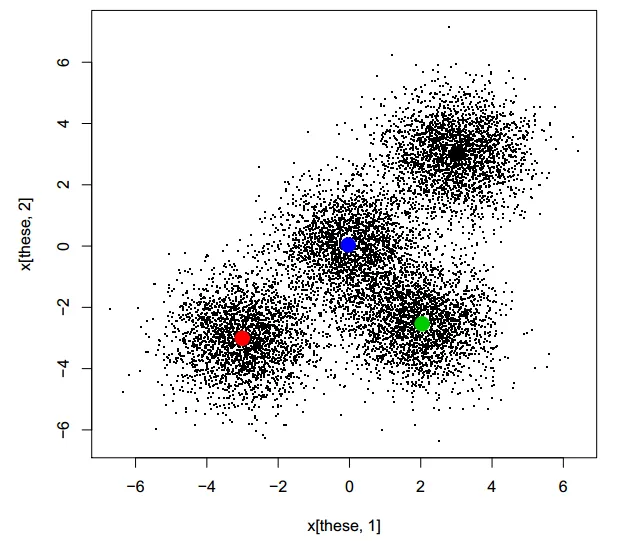
these <- sample(1:nrow(x), 10000)
plot(x[these,1], x[these,2], pch=".")
points(ans.kmeans$centers, pch=19, cex=2, col=1:4)
library(foreach)
library(doMC)
registerDoMC(3)
start.kmeans <- proc.time()[3]
ans.kmeans.par <- foreach(i=1:3) %dopar% {
return(kmeans(x, 4, nstart=1, iter.max=10, algorithm="Lloyd"))
}
TSS <- sapply(ans.kmeans.par, function(a) return(sum(a$withinss)))
ans.kmeans.par <- ans.kmeans.par[[which.min(TSS)]]
ans.kmeans.par$centers
end.kmeans <- proc.time()[3]
end.kmeans - start.kmeans
sink("mykmeans.Rfake")
kmeans
sink()
source("mykmeans.R")
start.kmeans <- proc.time()[3]
ans.kmeans <- mykmeans(x, 4, nstart=3, iter.max=10, algorithm="Lloyd")
ans.kmeans$centers
end.kmeans <- proc.time()[3]
end.kmeans - start.kmeans
x <- read.csv("Diving2000.csv", header=TRUE, as.is=TRUE)
library(YaleToolkit)
whatis(x)
x[1:14,c(3,6:9)]
meancol <- function(scores) {
temp <- matrix(scores, length(scores)/7, ncol=7)
means <- apply(temp, 1, mean)
ans <- rep(means,7)
return(ans)
}
x$panelmean <- meancol(x$JScore)
x[1:14,c(3,6:9,11)]
meancol <- function(scores) {
browser()
temp <- matrix(scores, length(scores)/7, ncol=7)
means <- apply(temp, 1, mean)
ans <- rep(means,7)
return(ans)
}
x$panelmean <- meancol(x$JScore)
以下是描述:
Number of cases: 10,787 scores from 1,541 dives (7 judges score each
dive) performed in four events at the 2000 Olympic Games in Sydney,
Australia.

Number of variables: 10.

Description: A full description and analysis is available in an
article in The American Statistician (publication details to be
announced).

Variables:

Event       Four events, men's and women's 3M and 10m.
Round       Preliminary, semifinal, and final rounds.
Diver       The name of the diver.
Country     The country of the diver.
Rank        The final rank of the diver in the event.
DiveNo      The number of the dive in sequence within round.
Difficulty  The degree of difficulty of the dive.
JScore      The score provided for the judge on this dive.
Judge       The name of the judge.
JCountry    The country of the judge.
并且提供数据集以进行实验 https://www.dropbox.com/s/urgzagv0a22114n/Diving2000.csv