如何将由geom_sf生成的地图放在由ggmap生成的栅格图像之上

Question

如何将由geom_sf生成的地图放在由ggmap生成的栅格图像之上

39

我尝试了以下代码:

library(ggplot2)
library(ggmap)
library(sf)
nc <- st_read(system.file("shape/nc.shp", package = "sf"))
str(nc)

 Classes ‘sf’ and 'data.frame':  100 obs. of  15 variables:
 $ AREA     : num  0.114 0.061 0.143 0.07 0.153 0.097 0.062 0.091 0.118 0.124 ...
 $ PERIMETER: num  1.44 1.23 1.63 2.97 2.21 ...
 $ CNTY_    : num  1825 1827 1828 1831 1832 ...
 $ CNTY_ID  : num  1825 1827 1828 1831 1832 ...
 $ NAME     : Factor w/ 100 levels "Alamance","Alexander",..: 5 3 86 27 66 46 15 37 93 85 ...
 $ FIPS     : Factor w/ 100 levels "37001","37003",..: 5 3 86 27 66 46 15 37 93 85 ...
 $ FIPSNO   : num  37009 37005 37171 37053 37131 ...
 $ CRESS_ID : int  5 3 86 27 66 46 15 37 93 85 ...
 $ BIR74    : num  1091 487 3188 508 1421 ...
 $ SID74    : num  1 0 5 1 9 7 0 0 4 1 ...
 $ NWBIR74  : num  10 10 208 123 1066 ...
 $ BIR79    : num  1364 542 3616 830 1606 ...
 $ SID79    : num  0 3 6 2 3 5 2 2 2 5 ...
 $ NWBIR79  : num  19 12 260 145 1197 ...
 $ geometry :sfc_MULTIPOLYGON of length 100; first list element: List of 1
 ..$ :List of 1
 .. ..$ : num [1:27, 1:2] -81.5 -81.5 -81.6 -81.6 -81.7 ...
   ..- attr(*, "class")= chr  "XY" "MULTIPOLYGON" "sfg"
   - attr(*, "sf_column")= chr "geometry"
   - attr(*, "agr")= Factor w/ 3 levels "constant","aggregate",..: NA NA NA NA NA NA NA NA NA NA ...
   ..- attr(*, "names")= chr  "AREA" "PERIMETER" "CNTY_" "CNTY_ID" ...

map <- get_map("north carolina", maptype = "satellite", zoom = 6, source = "google")
a <- unlist(attr(map,"bb")[1, ])
bb <- st_bbox(nc)
ggplot() + 
  annotation_raster(map, xmin = a[2], xmax = a[4], ymin = a[1], ymax = a[3]) + 
  xlim(c(bb[1], bb[3])) + ylim(c(bb[2], bb[4])) + 
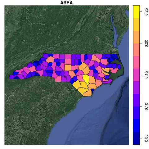
  geom_sf(data = nc, aes(fill = AREA))

这两层图层没有正确地重叠; 我尝试使用coord_sf() 更改投影，但没有成功。

有什么建议吗？谢谢

- user1453488

你能发布str(nc)的结果吗（编辑你的问题）？ - Phil

3个回答

17

你可以使用sf包中的绘图方法来完成这个任务。你需要指定坐标参考系统，我们需要假设（并且看起来确实如此）它是3857。

library(ggplot2)
library(ggmap)
library(sf)

nc_shp <- st_read(system.file("shape/nc.shp", package = "sf"))
nc_map <- get_map("north carolina", maptype = "satellite", zoom = 6, source = "google")

st_crs(nc_map)
# Coordinate Reference System: NA

# assume the coordinate refence system is 3857
plot(st_transform(nc_shp, crs = 3857)[1], bgMap = nc_map)

- Peter

可惜透明度不可得。 - undefined

0

所有的解决方案都很好，但是让我再添加一个对我有用的选项。

使用情况：将Tigris道路叠加到ggmap中

获取道路和边界（美国道路和俄亥俄州）：

US_roads <- primary_roads(); class(US_roads); OH_counties<-counties(state = "OH",year = 2018)
联合县来创建带有俄亥俄州边界的大几何体：

OH_poly <- st_union(OH_counties); plot(OH_poly)
在俄亥俄州内相交的道路

OH_roads<-st_intersection(US_roads,OH_poly); plot(OH_roads$geometry)
使用辅助函数将SF转换为SP以便于ggmap使用感兴趣的几何体（例如线或多边形）：

types <- vapply(sf::st_geometry(OH_roads), function(x) { class(x)[2] }, "")

OH_roads2 <- OH_roads[ grepl("*LINE", types), ]

OH_roads3<-as(OH_roads2, "Spatial")

OH_roads3<-as(OH_roads2, "空间")

OH_roads3@data$id <- OH_roads3@data$LINEARID
OH_roads4 <- fortify(OH_roads3, region='LINEARID')

绘制结果：

get_stamenmap(bbox, zoom = 10, maptype ="toner") %>% ggmap() + geom_path(data=OH_roads4, aes(long, lat,group = id),alpha=1,size=1,color="#c280e9",lineend = "round")

- Esteban M. Correa

网页内容由stack overflow 提供, 点击上面的

可以查看英文原文，
原文链接

- andyteucher · Accepted Answer

我自己也曾经遇到过这个问题，借助这篇文章的帮助，我找到了解决方法。 ggmap对象的边界框是在WGS84（EPSG：4326）中的，但实际光栅是在EPSG：3857中的。您必须修改ggmap对象的边界框，使其与底层数据具有相同的CRS：

library(ggplot2)
library(ggmap)
library(sf)
#> Linking to GEOS 3.6.2, GDAL 2.3.0, proj.4 5.1.0

nc <- st_read(system.file("shape/nc.shp", package = "sf"), quiet = TRUE)

# Transform nc to EPSG 3857 (Pseudo-Mercator, what Google uses)
nc_3857 <- st_transform(nc, 3857)

map <- get_map("north carolina", maptype = "satellite", zoom = 6, source = "google")

# Define a function to fix the bbox to be in EPSG:3857
ggmap_bbox <- function(map) {
  if (!inherits(map, "ggmap")) stop("map must be a ggmap object")
  # Extract the bounding box (in lat/lon) from the ggmap to a numeric vector, 
  # and set the names to what sf::st_bbox expects:
  map_bbox <- setNames(unlist(attr(map, "bb")), 
                       c("ymin", "xmin", "ymax", "xmax"))

  # Coonvert the bbox to an sf polygon, transform it to 3857, 
  # and convert back to a bbox (convoluted, but it works)
  bbox_3857 <- st_bbox(st_transform(st_as_sfc(st_bbox(map_bbox, crs = 4326)), 3857))

  # Overwrite the bbox of the ggmap object with the transformed coordinates 
  attr(map, "bb")$ll.lat <- bbox_3857["ymin"]
  attr(map, "bb")$ll.lon <- bbox_3857["xmin"]
  attr(map, "bb")$ur.lat <- bbox_3857["ymax"]
  attr(map, "bb")$ur.lon <- bbox_3857["xmax"]
  map
}

# Use the function:
map <- ggmap_bbox(map)

ggmap(map) + 
  coord_sf(crs = st_crs(3857)) + # force the ggplot2 map to be in 3857
  geom_sf(data = nc_3857, aes(fill = AREA), inherit.aes = FALSE)

这段文字是关于2018年6月13日使用reprex包（v0.2.0）创建的。