我想使用Python的谱聚类来对一个图进行聚类。
谱聚类是一种更通用的技术,不仅可以应用于图形,还可以应用于图像或任何类型的数据,但它被认为是一种特殊的图形聚类技术。不幸的是,我在网上找不到Python中关于谱聚类图形的示例。
Scikit Learn有两个文档记录的谱聚类方法:SpectralClustering和spectral_clustering,它们似乎不是别名。
这些方法都提到它们可以用于图形,但没有提供具体的指令。用户指南也没有。我已经向开发人员要求提供这样的示例,但他们工作繁忙,还没来得及处理。
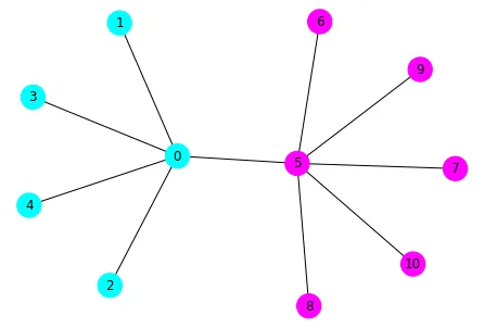
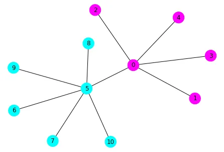
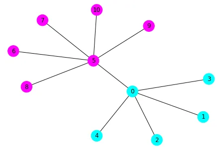
一个很好的网络用于记录这个问题是Karate Club网络。它已经包含在networkx的方法中。
我希望能得到一些指导来解决这个问题。如果有人能帮我弄清楚,我就可以把文档添加到Scikit Learn中。
SpectralClustering是一个面向对象的包装器,其中调用了spectral_clustering函数(以及其他内容)。https://stackoverflow.com/a/55720891/6509615 - rlchqrd