在Matlab中找到绘图上的点

Question

我有以下的图形和一个创建该图形的数据文件。我希望Matlab能够为我找到以下这些点：

1. 100%线所示峰值的[y,x]
2. 曲线与y=0线相交处的[x]
3. 在第1部分中找到的峰值的50％和20％处的[x]。

人们是否知道任何附加工具或软件包，可以帮助我完成这个任务？我需要对一系列的图像进行操作，因此自动化处理是理想的。

我当然可以在Matlab中完成编程和计算部分，只需要加载数据文件，匹配曲线或函数，并找到各种[x,y]坐标。

- Carl

---

图表看起来像数据集中只有几个点。如果是这样的话，图表中显示的线条只是实际数据点之间的线性插值。因此，获取50/20%的y值和y==0的x值将都是插值值...这确实是您想要的吗？ - Rody Oldenhuis

嗨，Rody。没错，对了。对于那些值进行插值将是可行的。我认为这将归结为近似高斯曲线或类似方法来匹配并估计各种值，是吗？ - Carl

那就是我的下一个问题了，你如何通过这些点进行插值会强烈影响所需的结果。我的意思是，如果你用直线进行插值（如上图所示），与使用25次多项式进行插值相比，你想要的结果将完全不同 :) 那么，你认为哪种插值方法最适合你的数据呢？ - Rody Oldenhuis

谢谢Rody。我认为用多项式会更好，因为这是一种自然信号，很可能会遵循曲线而不是直线。 - Carl

Answer 1

好的，下面开始。据我所知，Matlab中没有内置程序可以实现你想要的功能，你需要自己编写一个程序。需要注意的几个事项：

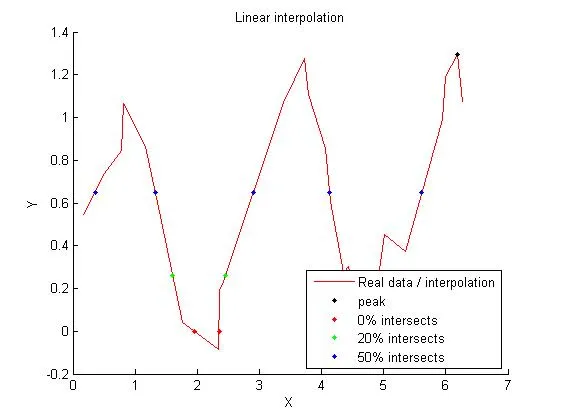
• 显而易见，线性插值数据最容易处理，也不应该有什么问题。

• 使用单一多项式插值也不太难，不过需要注意更多细节。首要任务是找到峰值，这涉及到找到导数的根（例如使用roots）。当找到峰值后，通过将多项式向上或向下偏移相应比例（0％，20％，50％），可以在所有所需级别上找到多项式的根。

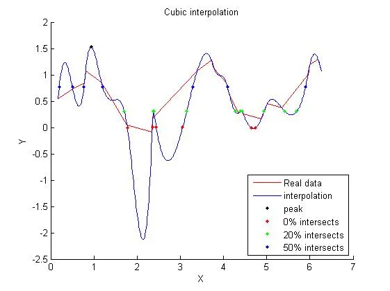
• 使用三次样条插值（spline）最为复杂。对于具有完整三阶段的所有子间隔，应重复上述用于一般多项式的例程，考虑到最大值也可能位于子间隔的边界上，并且任何找到的根和极值都可能在立方体有效的间隔之外（还要注意spline使用的x偏移量）。

这是我对所有三种方法的实现：

%% Initialize
% ---------------------------

clc
clear all

% Create some bogus data
n = 25;

f = @(x) cos(x) .* sin(4*x/pi) + 0.5*rand(size(x));
x = sort( 2*pi * rand(n,1));
y = f(x);


%% Linear interpolation
% ---------------------------

% y peak
[y_peak, ind] = max(y);
x_peak = x(ind);

% y == 0%, 20%, 50%
lims = [0 20 50];
X = cell(size(lims));
Y = cell(size(lims));
for p = 1:numel(lims)

    % the current level line to solve for
    lim = y_peak*lims(p)/100;

    % points before and after passing through the current limit
    after    = (circshift(y<lim,1) & y>lim) | (circshift(y>lim,1) & y<lim);
    after(1) = false;
    before   = circshift(after,-1);

    xx = [x(before) x(after)];
    yy = [y(before) y(after)];

    % interpolate and insert new data
    new_X = x(before) - (y(before)-lim).*diff(xx,[],2)./diff(yy,[],2);
    X{p} = new_X;
    Y{p} = lim * ones(size(new_X));

end

% make a plot to verify
figure(1), clf, hold on
plot(x,y, 'r') % (this also plots the interpolation in this case)

plot(x_peak,y_peak, 'k.') % the peak

plot(X{1},Y{1}, 'r.') % the 0%  intersects
plot(X{2},Y{2}, 'g.') % the 20% intersects
plot(X{3},Y{3}, 'b.') % the 50% intersects

% finish plot
xlabel('X'), ylabel('Y'), title('Linear interpolation')
legend(...
    'Real data / interpolation',...
    'peak',...
    '0% intersects',...
    '20% intersects',...
    '50% intersects',...
    'location', 'southeast')



%% Cubic splines
% ---------------------------

% Find cubic splines interpolation
pp = spline(x,y);

% Finding the peak requires finding the maxima of all cubics in all
% intervals. This means evaluating the value of the interpolation on 
% the bounds of each interval, finding the roots of the derivative and
% evaluating the interpolation on those roots: 

coefs = pp.coefs;
derivCoefs = bsxfun(@times, [3 2 1], coefs(:,1:3));
LB = pp.breaks(1:end-1).'; % lower bounds of all intervals
UB = pp.breaks(2:end).';   % upper bounds of all intervals

% rename for clarity
a = derivCoefs(:,1);
b = derivCoefs(:,2);  
c = derivCoefs(:,3); 

% collect and limits x-data
x_extrema = [...
    LB, UB,...     
    LB + (-b + sqrt(b.*b - 4.*a.*c))./2./a,... % NOTE: data is offset by LB
    LB + (-b - sqrt(b.*b - 4.*a.*c))./2./a,... % NOTE: data is offset by LB
    ];

x_extrema = x_extrema(imag(x_extrema) == 0);
x_extrema = x_extrema( x_extrema >= min(x(:)) & x_extrema <= max(x(:)) );

% NOW find the peak
[y_peak, ind] = max(ppval(pp, x_extrema(:)));
x_peak = x_extrema(ind);

% y == 0%, 20% and 50%
lims = [0 20 50];
X = cell(size(lims));
Y = cell(size(lims));    
for p = 1:numel(lims)

    % the current level line to solve for
    lim = y_peak * lims(p)/100;

    % find all 3 roots of all cubics
    R = NaN(size(coefs,1), 3); 
    for ii = 1:size(coefs,1) 

        % offset coefficients to find the right intersects
        C = coefs(ii,:);
        C(end) = C(end)-lim;

        % NOTE: data is offset by LB
        Rr = roots(C) + LB(ii); 

        % prune roots
        Rr( imag(Rr)~=0 ) = NaN;
        Rr( Rr <= LB(ii) | Rr >= UB(ii) ) = NaN;
        % insert results
        R(ii,:) = Rr;
    end

    % now evaluate and save all valid points    
    X{p} = R(~isnan(R));
    Y{p} = ppval(pp, X{p});

end

% as a sanity check, plot everything 
xx = linspace(min(x(:)), max(x(:)), 20*numel(x));
yy = ppval(pp, xx);

figure(2), clf, hold on

plot(x,y, 'r') % the actual data
plot(xx,yy) % the cubic-splines interpolation 

plot(x_peak,y_peak, 'k.') % the peak

plot(X{1},Y{1}, 'r.') % the 0%  intersects
plot(X{2},Y{2}, 'g.') % the 20% intersects
plot(X{3},Y{3}, 'b.') % the 50% intersects

% finish plot
xlabel('X'), ylabel('Y'), title('Cubic splines interpolation')
legend(...
    'Real data',...
    'interpolation',...
    'peak',...
    '0% intersects',...
    '20% intersects',...
    '50% intersects',...
    'location', 'southeast')


%% (N-1)th degree polynomial
% ---------------------------

% Find best interpolating polynomial
coefs = bsxfun(@power, x, n-1:-1:0) \ y;
% (alternatively, you can use polyfit() to do this, but this is faster)

% To find the peak, we'll have to find the roots of the derivative: 
derivCoefs = (n-1:-1:1).' .* coefs(1:end-1);
Rderiv = roots(derivCoefs);
Rderiv = Rderiv(imag(Rderiv) == 0);
Rderiv = Rderiv(Rderiv >= min(x(:)) &  Rderiv <= max(x(:)));

[y_peak, ind] = max(polyval(coefs, Rderiv));
x_peak = Rderiv(ind);

% y == 0%, 20%, 50%
lims = [0 20 50];
X = cell(size(lims));
Y = cell(size(lims));
for p = 1:numel(lims)

    % the current level line to solve for
    lim = y_peak * lims(p)/100;

    % offset coefficients as to find the right intersects
    C = coefs;
    C(end) = C(end)-lim;

    % find and prune roots
    R = roots(C);
    R = R(imag(R) == 0);
    R = R(R>min(x(:)) & R<max(x(:)));

    % evaluate polynomial at these roots to get actual data
    X{p} = R;
    Y{p} = polyval(coefs, R);

end

% as a sanity check, plot everything 
xx = linspace(min(x(:)), max(x(:)), 20*numel(x));
yy = polyval(coefs, xx);

figure(3), clf, hold on

plot(x,y, 'r') % the actual data
plot(xx,yy) % the cubic-splines interpolation 

plot(x_peak,y_peak, 'k.') % the peak

plot(X{1},Y{1}, 'r.') % the 0%  intersects
plot(X{2},Y{2}, 'g.') % the 20% intersects
plot(X{3},Y{3}, 'b.') % the 50% intersects

% finish plot
xlabel('X'), ylabel('Y'), title('(N-1)th degree polynomial')
legend(...
    'Real data',...
    'interpolation',...
    'peak',...
    '0% intersects',...
    '20% intersects',...
    '50% intersects',...
    'location', 'southeast')

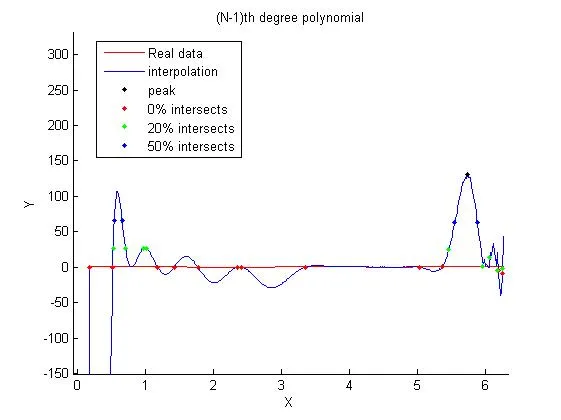
这将导致三个图表： （请注意，在（N-1）次多项式中会出现一些问题；20％的交叉点在末尾都是错误的。因此，在复制粘贴之前，请更加仔细地检查一切 :)）

正如我之前所说，也正如您可以清楚地看到的那样，如果底层数据不适合单个多项式进行插值，则单个多项式进行插值通常会引入许多问题。而且，正如您可以从这些图表清楚地看到的那样，插值方法非常强烈地影响交点的位置 - 最重要的是，您必须至少有一些关于底层数据模型的想法。

对于一般情况，三次样条通常是最好的选择。然而，这是一种通用方法，并会给您（以及您的出版物读者）带来对数据准确性的虚假感知。使用三次样条获得有关相交点及其行为的第一个想法，但是一旦真实模型变得更加清晰，一定要回来重新审查您的分析。当只用于通过数据创建更平滑、更“视觉上吸引人”的曲线时，请勿使用三次样条进行发布 :)

- Rody Oldenhuis

---

这是一个非常好的答案。非常感谢您提供了详细的解释和注意事项。我已经开始阅读并且正好满足了我所需求的。谢谢。 - Carl

Answer 2

使用 MAX 函数来寻找全局最大值：

[ymax, imax] = max(y);
xmax = x(imax);
line(xlim,[ymax ymax],'Color','r')
line(xmax,ymax,'Color','r','LineStyle','o')

对于剩下的部分，您可以使用出色的FileExchange提交 - "快速而强大的曲线交点"。

在y = 0处定义线条可以使用xlim和yline0 = [0 0];。 然后您可以执行以下操作

[x0, y0] = intersections(x,y,xlim,yline0); % function from FileExchange
x0close(1) = xmax - min(xmax-x0(x0<xmax));
x0close(2) = xmax + min(x0(x0>xmax)-xmax);
y0close = y0(ismember(x0,x0close));
line(xlim,yline0,'Color','r')
line(x0close,y0close,'Color','r','LineStyle','o')

同样的操作也可以针对20%和50%，除此之外

。

yline20 = repmat((ymax - y0(1))*0.2,1,2);

---

这一切都假设您想要直线的交点，就像您的图表上那样，而不是插值。

- yuk

Answer 3

这不是完整的答案，但Matlab有内置函数可以完成大部分你想做的事情。

• max可以帮助你找到100%线。
• polyfit将以最小二乘意义给出一组点的多项式拟合。如果你想让它穿过n个点，我认为你需要至少使用n-1次幂。
• roots将给出你刚刚找到的多项式的零点交叉。你也可以通过减去一个常数来找到20%和50%的交叉点。当存在多个交叉点时，你会想要选择距离你最初找到的最大值最近的那些。(你确定交叉点总是存在吗？)

- nhowe