Matlab: "X-Ray" 通过补丁绘制线条

Question

Matlab: "X-Ray" 通过补丁绘制线条

3

问题

我想要可视化一条3D路径，并围绕它形成一个代表数据标准差的“云” 。我想让路径呈现为一条黑色粗线，周围均匀灰色区域，没有任何云雾状线条，就像透过云层的X光线看到的线条一样。

尝试 Attempt 1

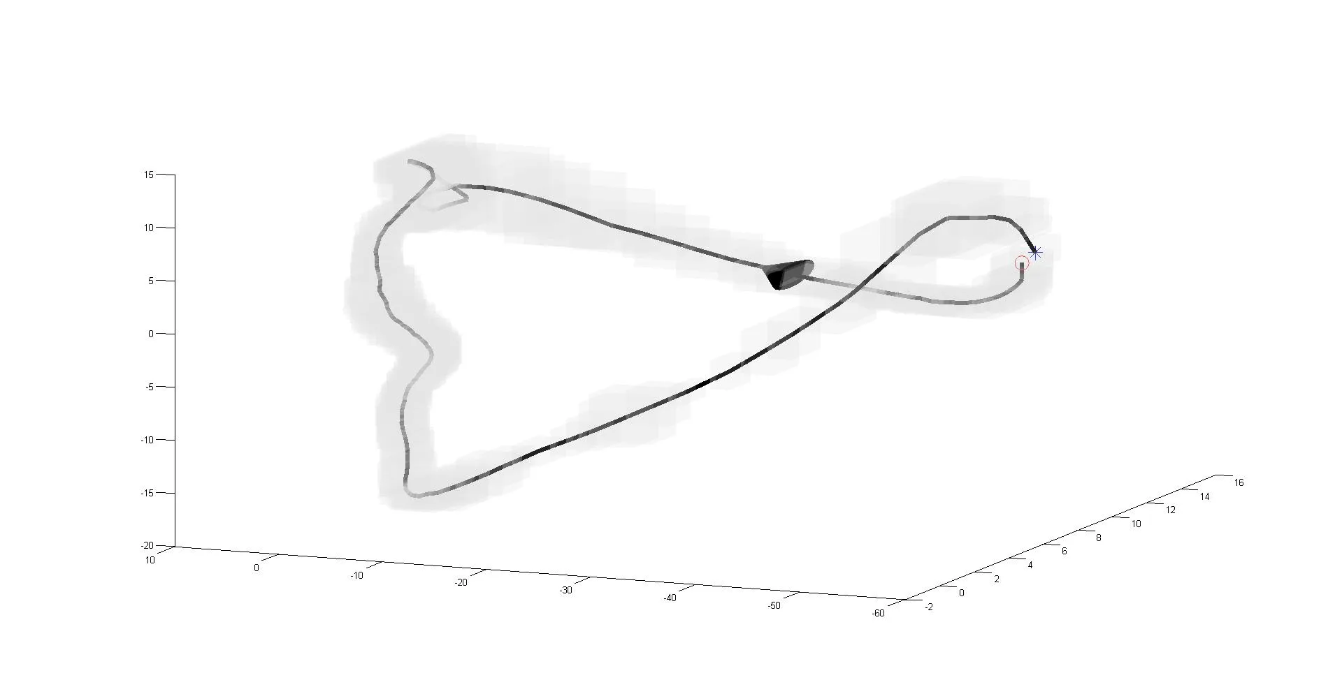
我使用plot3创建了一条粗线，使用patch在每个线段的中心点创建了一系列方块（图中还有一些额外的东西表示开始/结束和方向，我也希望它们容易被看到）。我尝试调整patch的alpha，但是会在线条上产生云雾状效果，使得灰色颜色的亮度随着视线中有多少个灰色盒子而变化。我希望alpha值为1，以便每个灰色方块的颜色都完全相同，但我希望找到一种方法使线条通过云层时更均匀地显示。

最小示例

如所请求，这里是一个最小示例，生成下面的绘图。 Example 2

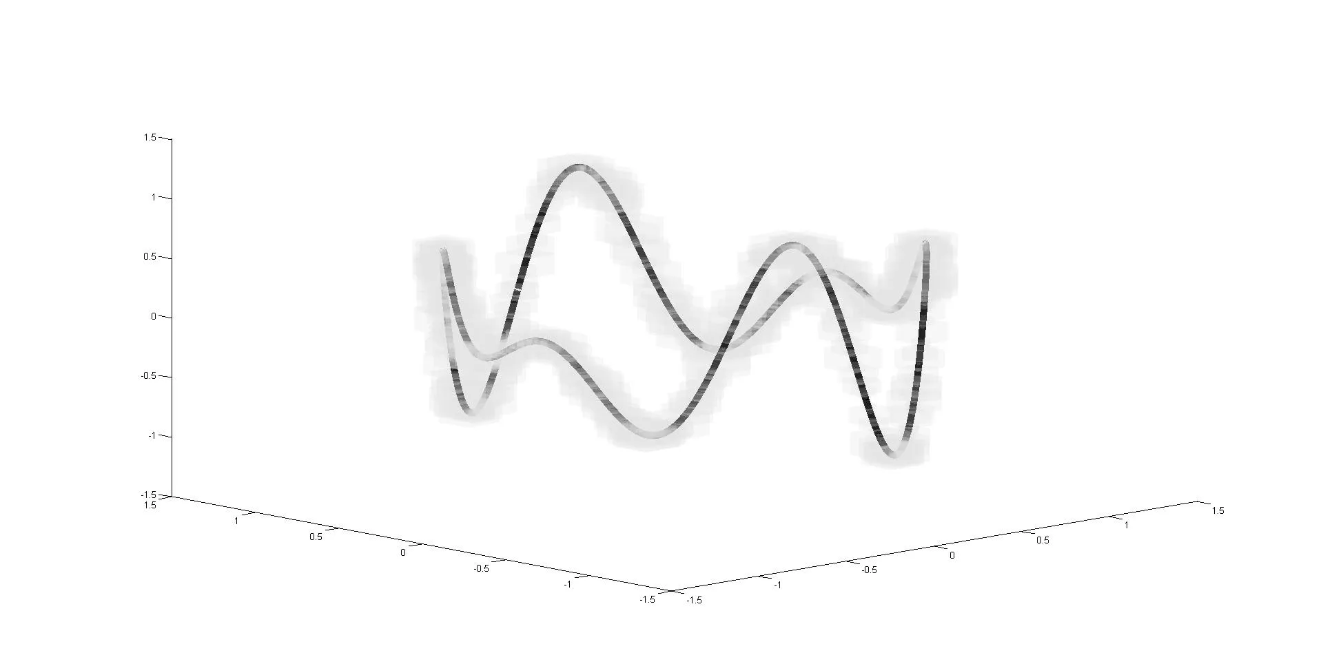
% Create a path as an example (a circle in the x-y plane, with sinusoidal deviations in the z-axis)
t = 0:1/100:2*pi;
x = sin(t);y = cos(t);
z = cos(t).*sin(5*t);
figure;
plot3(x,y,z,'k','linewidth',7);

% Draw patches
cloud = .1*rand(size(t)); % The size of each box (make them random, "like" real data)
grayIntensity = .9; % Color of patch
faceAlpha = .15; % Alpha of patch

for i = 1:length(x)
patch([x(i) - cloud(i); x(i) + cloud(i); x(i) - cloud(i); x(i) + cloud(i); x(i) - cloud(i); x(i) + cloud(i); x(i) - cloud(i); x(i) + cloud(i)],... % X values
[y(i) - cloud(i); y(i) - cloud(i); y(i) + cloud(i); y(i) + cloud(i); y(i) - cloud(i); y(i) - cloud(i); y(i) + cloud(i); y(i) + cloud(i)],... % Y values
[z(i) + cloud(i); z(i) + cloud(i); z(i) + cloud(i); z(i) + cloud(i); z(i) - cloud(i); z(i) - cloud(i); z(i) - cloud(i); z(i) - cloud(i)],... % Z values
grayIntensity*ones(1,3),... % Color of patch
'faces', [1 2 4 3;5 6 8 7;1 2 6 5; 8 7 3 4;1 5 7 3;2 6 8 4],... % Connect vertices to form faces (a box)
'edgealpha',0,... % Make edges invisible (to get continuous cloud effect)
'facealpha',faceAlpha); % Set alpha of faces
end

很抱歉for loop中有非常长的代码段，patch命令有相当多的参数。前三行只是通过指定中心点加上或减去立方体的一半宽度cloud(i)来定义8个顶点的x、y和z坐标。其余部分应根据各自的注释说明。

感谢您的任何帮助！

- sgbrown

我认为（不确定）你可以使用zbuffer渲染模式来实现这个。所以你可以使用set(gca,'Renderer','zbuffer')，先绘制灰色的东西，然后再绘制黑色的。我不确定它是否会起作用，但是可能会... - Ander Biguri

1

我曾经遇到过类似的问题。我通过创建一个表面来解决它，该表面代表您的云的包络（由中心线上所有圆盘/盒子定义）。然后，您只需要管理一个对象，许多对象的alpha值不会相加，因此主中心线非常清晰可见。但是，您需要提供更多数据才能将其应用于您的情况。 - Hoki

1

@AnderBiguri，思路不错。我尝试了你的解决方案，但它只适用于2D。在3D中，即使将线的手柄放在uistack的顶部（或最后绘制），渲染器也会检测到线的“后面”部分（相对于相机）并且不会为这些隐藏的部分渲染线条（完全不渲染）。 - Hoki

@Hoki 没错。我试图查看是否有一种方法可以仅禁用Z缓冲区，就像在使用OpenGL时那样，但我找不到这样的方法... - Ander Biguri

@Hoki 这是个好主意，但是试图将我的“云”简化为单一的表面可能有些复杂。不过，如果没有其他办法，我会尝试的，谢谢！ - sgbrown

2个回答

1

这是我在评论中提到的解决方案的实现（仅绘制一个单一的surface云）。

它没有进行优化，有一些for循环可以通过巧妙地使用bsxfun或这些辅助函数来避免，但它可以正常运行。每个点上找到曲线的切线并定向（旋转）每个横截面的数学可能也可以简化，但这不是我的强项，所以如果专家们觉得需要的话，就留给他们去做吧。

基本上，它定义了一个圆（通常在代码中称为“横截面”），其半径与某个东西成比例（在您的应用程序中为标准偏差，在示例中为随机值）。然后，将每个圆在3D中旋转，使其垂直于它被翻译的点处的曲线。所有这些圆都被用作单个surface图形对象的信封。

当表面重叠多次时（取决于视角），主中心线仍会有些阴影，但主要线始终可见。此外，您只需要管理一个图形对象。

结果看起来像这样：

当然，您可以根据自己的喜好改变表面的AlphaValue。我定义了一个与数据大小相同的完整矩阵来存储颜色信息。目前它全部设置为0（因此指向默认colormap中的绿色），但这样如果您想使颜色函数依赖于其他参数，只需相应地调整颜色矩阵（以及相关的colormap）即可。

代码末尾有一个选项，可以将每个横截面显示为一个patch object。这不是最终结果的意图，但如果您想进行自己的修改并理解整个构造过程，它会很有帮助。

以下是代码：

%% // Create a path as an example (a circle in the x-y plane, with sinusoidal deviations in the z-axis)
nPts = 180 ;
t = linspace(0,359,nPts)*pi/180;
x = sin(t); y = cos(t);
z = cos(t).*sin(2*t);

figure;
h.line = plot3(x,y,z,'k','linewidth',2,'Marker','none');
hold on
xlabel('X')
ylabel('Y')
zlabel('Z')

%% // Define options
%// cloud = .1*rand(size(t)) ; % The size of each box (make them random, "like" real data)
%// I used another randomization process, make that function of your stdev
r.min = 0.1 ; r.max = 0.2 ;
radius = r.min + (r.max-r.min).* rand(size(t)) ;

%// define surface and patch display options (FaceAlpha etc ...), for later
surfoptions  = {'FaceAlpha',0.2 , 'EdgeColor','none' , 'EdgeAlpha',0.1 , 'DiffuseStrength',1 , 'AmbientStrength',1 } ;
patchoptions = {'FaceAlpha',0.2 , 'EdgeColor','k'    , 'EdgeAlpha',0.2 , 'DiffuseStrength',1 , 'AmbientStrength',1 } ;
patchcol     = [1 0 0] ;  % Color of patch

%% // get the gradient at each point of the curve
Gx = diff([x,x(1)]).' ;                       %'//damn StackOverflow prettifier 
Gy = diff([y,y(1)]).' ;                       %'//damn StackOverflow prettifier 
Gz = diff([z,z(1)]).' ;                       %'//damn StackOverflow prettifier 
%// get the middle gradient between 2 segments (optional, just for better rendering if low number of points)
G = [ (Gx+circshift(Gx,1))./2 (Gy+circshift(Gy,1))./2 (Gz+circshift(Gz,1))./2] ;

%% // get the angles (azimuth, elevation) of each plane normal to the curve

ux = [1 0 0] ;
uy = [0 1 0] ;
uz = [0 0 1] ;

for k = nPts:-1:1 %// running the loop in reverse does automatic preallocation
    a = G(k,:) ./ norm(G(k,:)) ;
    angx(k) =  atan2( norm(cross(a,ux)) , dot(a,ux))  ;
    angy(k) =  atan2( norm(cross(a,uy)) , dot(a,uy))  ;
    angz(k) =  atan2( norm(cross(a,uz)) , dot(a,uz))  ;

    [az(k),el(k)] = cart2sph( a(1) , a(2) , a(3) ) ;
end
%// adjustment to be normal to cross section plane the way the rotation are defined later
az = az + pi/2 ; 
el = pi/2 - el ;

%% // define basic disc
discResolution = 20 ;
tt = linspace( 0 , 2*pi , discResolution ) ;
xd = cos(tt) ;
yd = sin(tt) ;
zd = zeros( size(xd) ) ;

%% // Generate coordinates for each cross section

ccylX = zeros( nPts , discResolution ) ;
ccylY = zeros( nPts , discResolution ) ;
ccylZ = zeros( nPts , discResolution ) ;
ccylC = zeros( nPts , discResolution ) ;

for ip = 1:nPts
    %// cross section coordinates, with radius function of [rand] in this
    %// example. Make it function of the stdev in your application.
    csTemp = [ ( radius(ip) .* xd )  ; ... %// X coordinates
               ( radius(ip) .* yd )  ; ... %// Y coordinates
                               zd    ] ;   %// Z coordinates

    %// rotate the cross section (around X axis, around origin)
    elev = el(ip) ;
    Rmat = [ 1     0           0     ; ...
             0 cos(elev)  -sin(elev) ; ...
             0 sin(elev)   cos(elev) ] ;
    csTemp = Rmat * csTemp ;

    %// do the same again to orient the azimuth (around Z axis)
    azi = az(ip) ;
    Rmat = [ cos(azi)  -sin(azi) 0 ; ...
             sin(azi)   cos(azi) 0 ; ...
               0            0    1 ] ;
    csTemp = Rmat * csTemp ;

    %// translate each cross section where it should be and store in global coordinate vector
    ccylX(ip,:) = csTemp(1,:) + x(ip) ;
    ccylY(ip,:) = csTemp(2,:) + y(ip) ;
    ccylZ(ip,:) = csTemp(3,:) + z(ip) ;
end

%% // Display the full cylinder
hd.cyl = surf( ccylX , ccylY , ccylZ , ccylC ) ;

%// use that if the graphic object already exist but you just want to update your data:
%// set( hd.cyl , 'XData',ccylX , 'YData',ccylY ,'ZData',ccylZ ) 

set( hd.cyl , surfoptions{:} )


%% // this is just to avoid displaying the patches in the next block
%// comment the "return" instruction or just execute next block if you want
%// to see the building cross sections as patches
return 

%% // display patches
hp = zeros(nPts,1) ;
for ip = 1:nPts
   hp(ip) = patch( ccylX(ip,:) , ccylY(ip,:) , ccylZ(ip,:) , patchcol ) ;
   set( hp(ip) , patchoptions{:} )
end

这只是一个带有补丁的快速缩放视图（代码重新运行，点数较低，否则会很快混乱整个图形）：

cloudenvzoom

- Hoki

谢谢您阐述观点！虽然它仍然有一些我最初代码的问题，但是它看起来比我原先的代码整洁了几个数量级，而且对于我的使用来说将是完美的。再次感谢您明显花费在您的想法和示例上的时间！ - sgbrown

网页内容由stack overflow 提供, 点击上面的

可以查看英文原文，
原文链接

- le_sacre · Accepted Answer

我的Matlab版本比较老，但是类似下面的代码可能对你也有帮助：

Draw the cloudy patches first as you did above (not the solid path yet).
Store the axis handle:
```
patch_axis = gca;
```

Create a new, overlapping axis:

path_axis = axes('position',get(patch_axis,'position'),'visible','off');

Draw the solid path line (in this new axis).

Link rotation and limits of the patch_axis (behind) to that of the path_axis (in front):

set(rotate3d(path_axis),'ActionPostCallback', ...
@(src,evt)set(patch_axis,{'view','xlim','ylim','zlim'}, ...
get(path_axis,{'view','xlim','ylim','zlim'})));

If you are rotating your view manually then it should line up the two axes after your first adjustment and keep them lined up. But if you're setting the rotation and limits with a command, then you can either just include both axis handles (patch_axis & path_axis) in your set command or copy the settings after:
```
set(patch_axis,{'view','xlim','ylim','zlim'}, ...
get(path_axis,{'view','xlim','ylim','zlim'})
```

请注意，要调整轴属性（刻度标签等），您需要对可见的patch_axis进行操作，而不是不可见的path_axis。如果您希望它在手动旋转时实时交互，我不确定如何使对齐函数在每次重绘时执行。