刚开始了解时间序列,并使用这篇R-bloggers文章作为下面的练习指导:企图预测股市未来回报率...只是理解时间序列概念的练习。
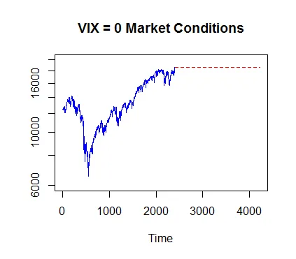
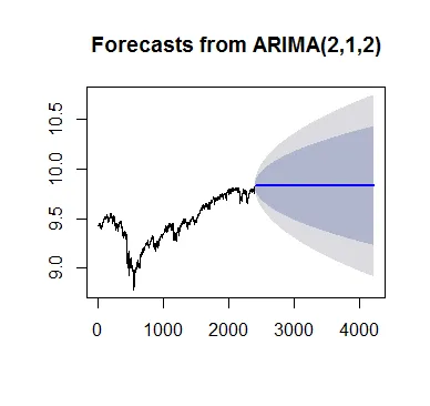
问题在于,当我绘制预测值时,得到的是一条常数线,与历史数据不符。下面是它在平稳化后的历史道琼斯日回报率的尾部的蓝色线。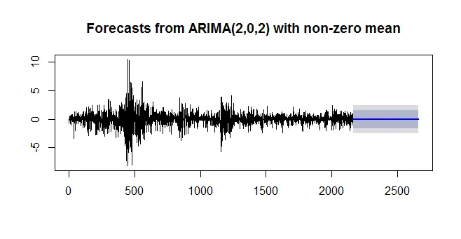 实际上,我想要更加“乐观”的视觉效果,或者是一个“重新趋势化”的绘图,就像我对航空旅客预测数量所得到的那个:
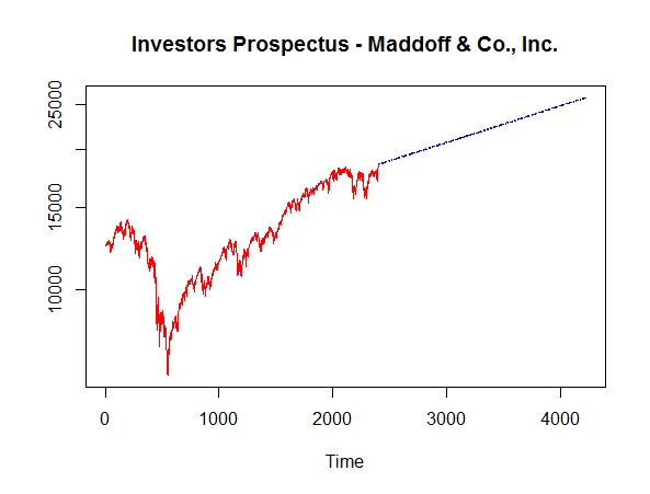
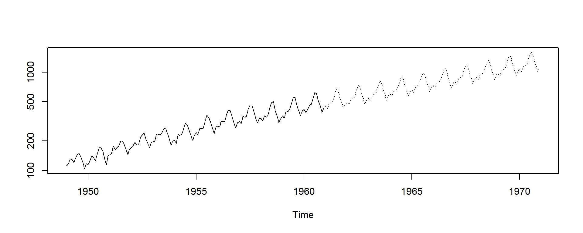
 以下是代码:
应用于当前问题的解决方案可能是这样的:
问题在于,当我绘制预测值时,得到的是一条常数线,与历史数据不符。下面是它在平稳化后的历史道琼斯日回报率的尾部的蓝色线。
实际上,我想要更加“乐观”的视觉效果,或者是一个“重新趋势化”的绘图,就像我对航空旅客预测数量所得到的那个:
以下是代码:library(quantmod)
library(tseries)
library(forecast)
getSymbols("^DJI")
d = DJI$DJI.Adjusted
chartSeries(DJI)
adf.test(d)
dow = 100 * diff(log(d))[-1]
adf.test(dow)
train = dow[1 : (0.9 * length(dow))]
test = dow[(0.9 * length(dow) + 1): length(dow)]
fit = arima(train, order = c(2, 0, 2))
predi = predict(fit, n.ahead = (length(dow) - (0.9*length(dow))))$pred
fore = forecast(fit, h = 500)
plot(fore)
很不幸,如果我尝试将同样的代码用于航空旅客预测,就会出现错误。例如:
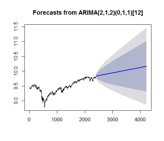
fit = arima(log(AirPassengers), c(0, 1, 1), seasonal = list(order = c(0, 1, 1), period = 12))
pred <- predict(fit, n.ahead = 10*12)
ts.plot(AirPassengers,exp(pred$pred), log = "y", lty = c(1,3))
应用于当前问题的解决方案可能是这样的:
fit2 = arima(log(d), c(2, 0, 2))
pred = predict(fit2, n.ahead = 500)
ts.plot(d,exp(pred$pred), log = "y", lty = c(1,3))
Error in .cbind.ts(list(...), .makeNamesTs(...), dframe = dframe, union = TRUE) : non-time series not of the correct length