使用R语言进行近距离地图制作

Question

我想用R创建一些接近度图，显示某些点离不同区域的距离。我找不到任何R代码示例，但我找到了一个输出结果，它是我想要的类型: 。

这个图并不一定需要所有标签和内部边界的魔法，但我希望它能在海岸边界停止(考虑使用'rgeos'函数'gintersection' - 参见这里)。

我尝试做密度图作为'热力图'(这将是一个相当不错的解决方案/替代方案)，并在上面放置一个shapefile(按照这个建议suggestion)，但它们没有对齐，我不能做一个'gintersection'，可能是因为密度图没有与之相关联的坐标系。

- cs234

---

你可以使用rgeos函数gBuffer()来完成此操作。这份文档提供了一个很好的例子：http://www.nickeubank.com/wp-content/uploads/2015/10/RGIS2_MergingSpatialData_part2_GeometricManipulations.html - tktk234

Answer 1

我用你的问题试着使用新的库进行了一些操作...

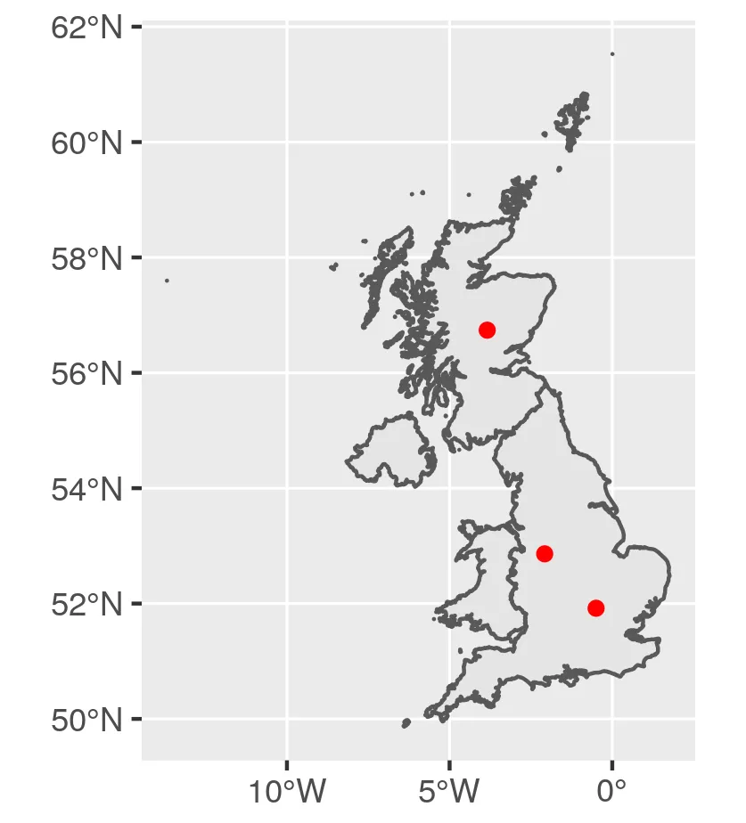
获取英国地图并定义随机点

library(raster)
library(sf)
library(ggplot2)
library(dplyr)
library(tidyr)
library(forcats)
library(purrr)

# Get UK map
GBR <- getData(name = "GADM", country = "GBR", level = 1)
GBR_sf <- st_as_sf(GBR)

# Define 3 points on the UK map
pts <- matrix(c(-0.4966766, -2.0772529, -3.8437793, 
                51.91829, 52.86147, 56.73899), ncol = 2)
# Project in mercator to allow buffer with distances
pts_sf <- st_sfc(st_multipoint(pts), crs = 4326) %>% 
  st_sf() %>%
  st_transform(27700)

ggplot() +
  geom_sf(data = GBR_sf) +
  geom_sf(data = pts_sf, colour = "red")

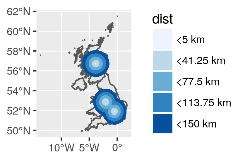
计算缓冲区域

我们为每个缓冲距离创建一个 multipolygons 列表。由于缓冲距离是基于坐标系的比例尺来计算的，因此点数据集必须使用投影坐标（这里是墨卡托）。

# Define distances to buffer
dists <- seq(5000, 150000, length.out = 5)
# Create buffer areas with each distances
pts_buf <- purrr::map(dists, ~st_buffer(pts_sf, .)) %>%
  do.call("rbind", .) %>% 
  st_cast() %>%
  mutate(
    distmax = dists,
    dist = glue::glue("<{dists/1000} km"))
# Plot: alpha allows to see overlapping polygons
ggplot() +
  geom_sf(data = GBR_sf) +
  geom_sf(data = pts_buf, fill = "red",
          colour = NA, alpha = 0.1)

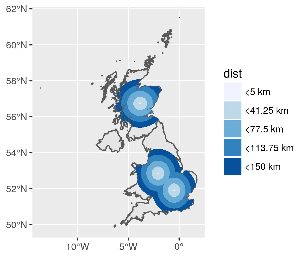
去除重叠

缓冲区域重叠。在上图中，更强烈的红色是由于透明红色的多层重叠造成的。让我们去掉重叠部分。我们需要从较大的区域中删除尺寸较小的缓冲区。然后，我需要将最小的区域再次添加到列表中。

# Remove part of polygons overlapping smaller buffer
pts_holes <- purrr::map2(tail(1:nrow(pts_buf),-1),
            head(1:nrow(pts_buf),-1),
            ~st_difference(pts_buf[.x,], pts_buf[.y,])) %>%
  do.call("rbind", .) %>% 
  st_cast() %>%
  select(-distmax.1, -dist.1)
# Add smallest polygon
pts_holes_tot <- pts_holes %>% 
  rbind(filter(pts_buf, distmax == min(dists))) %>%
  arrange(distmax) %>%
  mutate(dist = forcats::fct_reorder(dist, distmax))
# Plot and define color according to dist
ggplot() +
  geom_sf(data = GBR_sf) +
  geom_sf(data = pts_holes_tot,
          aes(fill = dist),
          colour = NA) +
  scale_fill_brewer(direction = 2)

删除海洋区域

如果您只想在陆地上查找邻近区域，则需要删除位于海洋中的缓冲区域。使用相同投影的多边形之间进行交集计算。我之前对英国地图进行了联合处理。

# Remove part of polygons in the sea
# Union and projection of UK map
GBR_sf_merc <- st_transform(st_union(GBR_sf), 27700)
pts_holes_uk <- st_intersection(pts_holes_tot, 
                              GBR_sf_merc)

ggplot() +
  geom_sf(data = GBR_sf) +
  geom_sf(data = pts_holes_uk,
          aes(fill = dist),
          colour = NA) +
  scale_fill_brewer(direction = 2)

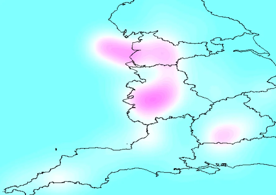
这是使用sf、ggplot2和其他几个库创建的最终接近度地图...

- Sébastien Rochette

Answer 2

在Sébastien的示例基础上，我们可以采用更传统的方法：

library(raster)
GBR <- getData(name = "GADM", country = "GBR", level = 1)
pts <- matrix(c(-0.4966766, -2.0772529, -3.8437793, 51.91829, 52.86147, 56.73899), ncol = 2)

r <- raster(GBR, res=1/12)
d <- distanceFromPoints(r, pts)
m <- mask(d, GBR)

plot(m)

- Robert Hijmans

---

这应该是答案。 - Thomas