在PyMC3中运行多元有序logit模型

Question

我正在尝试使用PyMC3构建Bayesian多元有序logit模型。我已经成功地基于这本书中的示例创建了一个玩具多元logit模型。我也已经根据此页面底部的示例实现了有序逻辑回归模型。

但是，我无法运行有序的多元逻辑回归。我认为问题可能在于切点的指定方式，具体来说是形状参数，但我不确定为什么如果有多个独立变量就会与只有一个变量时有所不同，因为响应类别的数量并没有改变。

以下是我的代码：

MWE的数据准备：

import pymc3 as pm
import numpy as np
import pandas as pd
from sklearn.datasets import load_iris

iris = load_iris(return_X_y=False)
iris = pd.DataFrame(data=np.c_[iris['data'], iris['target']],
                     columns=iris['feature_names'] + ['target'])

iris = iris.rename(index=str, columns={'sepal length (cm)': 'sepal_length', 'sepal width (cm)': 'sepal_width', 'target': 'species'})

这是一个可用的多元（二元）逻辑回归：

df = iris.loc[iris['species'].isin([0, 1])]
y = pd.Categorical(df['species']).codes
x = df[['sepal_length', 'sepal_width']].values

with pm.Model() as model_1:
      alpha = pm.Normal('alpha', mu=0, sd=10)
      beta = pm.Normal('beta', mu=0, sd=2, shape=x.shape[1])
      mu = alpha + pm.math.dot(x, beta)
      theta = 1 / (1 + pm.math.exp(-mu))
      y_ = pm.Bernoulli('yl', p=theta, observed=y)
      trace_1 = pm.sample(5000)

下面是一个使用有序logit回归（只含有一个自变量）的有效示例：

x = iris['sepal_length'].values
y = pd.Categorical(iris['species']).codes

with pm.Model() as model:
    cutpoints = pm.Normal("cutpoints", mu=[-2,2], sd=10, shape=2,
                          transform=pm.distributions.transforms.ordered)

    y_ = pm.OrderedLogistic("y", cutpoints=cutpoints, eta=x, observed=y)
    tr = pm.sample(1000)

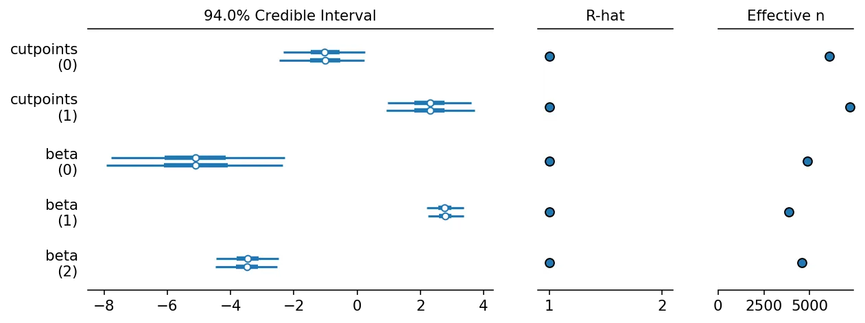
这是我尝试实现的多元有序Logit模型，它可以分解：

x = iris[['sepal_length', 'sepal_width']].values
y = pd.Categorical(iris['species']).codes

with pm.Model() as model:
    cutpoints = pm.Normal("cutpoints", mu=[-2,2], sd=10, shape=2,
                          transform=pm.distributions.transforms.ordered)

    y_ = pm.OrderedLogistic("y", cutpoints=cutpoints, eta=x, observed=y)
    tr = pm.sample(1000)

我收到的错误消息是：“ValueError: all the input array dimensions except for the concatenation axis must match exactly.” 这表明这是一个数据问题（x, y），但数据看起来与多元逻辑回归相同，后者可以正常运行。

如何修复有序多元逻辑回归以使其正常运行？

- Maya

Answer 1

我之前从未做过多元有序回归。但似乎有两种方法来解决模型问题：

1.在预测空间中划分，这种情况下，你需要使用切割线/曲线而不是点。

2.在转换的空间中进行分区，在此空间中，您已将预测空间投影到一个标量值，并可以再次使用切割点。

如果要使用pm.OrderedLogistic，则似乎必须采用后者，因为它似乎不支持开箱即用的多元eta情况。

这是我的尝试，但我不确定这是否是一种标准方法。

import numpy as np
import pymc3 as pm
import pandas as pd
import theano.tensor as tt
from sklearn.datasets import load_iris

# Load data
iris = load_iris(return_X_y=False)
iris = pd.DataFrame(data=np.c_[iris['data'], iris['target']],
                     columns=iris['feature_names'] + ['target'])
iris = iris.rename(index=str, columns={
    'sepal length (cm)': 'sepal_length', 
    'sepal width (cm)': 'sepal_width', 
    'target': 'species'})

# Prep input data
Y = pd.Categorical(iris['species']).codes
X = iris[['sepal_length', 'sepal_width']].values

# augment X for simpler regression expression
X_aug = tt.concatenate((np.ones((X.shape[0], 1)), X), axis=1)

# Model with sampling
with pm.Model() as ordered_mvlogit:
    # regression coefficients
    beta = pm.Normal('beta', mu=0, sd=2, shape=X.shape[1] + 1)

    # transformed space (univariate real)
    eta = X_aug.dot(beta)

    # points for separating categories
    cutpoints = pm.Normal("cutpoints", mu=np.array([-1,1]), sd=1, shape=2,
                          transform=pm.distributions.transforms.ordered)

    y_ = pm.OrderedLogistic("y", cutpoints=cutpoints, eta=eta, observed=Y)

    trace_mvordlogit = pm.sample(5000)

这个似乎收敛很好，生成了不错的间隔。

如果你把 beta 和 cutpoint 的均值回计算到预测空间中，就会得到以下分区，看起来合理。 不过，花萼长度和宽度并不是最适合分区的特征。

# Extract mean parameter values
b0, b1, b2 = trace_mvordlogit.get_values(varname='beta').mean(axis=0)
cut1, cut2 = trace_mvordlogit.get_values(varname='cutpoints').mean(axis=0)

# plotting parameters
x_min, y_min = X.min(axis=0)
x_max, y_max = X.max(axis=0)

buffer = 0.2
num_points = 37

# compute grid values
x = np.linspace(x_min - buffer, x_max + buffer, num_points)
y = np.linspace(y_min - buffer, y_max + buffer, num_points)

X_plt, Y_plt = np.meshgrid(x, y)
Z_plt = b0 + b1*X_plt + b2*Y_plt

# contour + scatter plots
plt.figure(figsize=(8,8))
plt.contourf(X_plt,Y_plt,Z_plt, levels=[-80, cut1, cut2, 50])
plt.scatter(iris.sepal_length, iris.sepal_width, c=iris.species)
plt.xlabel("Sepal Length")
plt.ylabel("Sepal Width")
plt.show()

二阶项

您可以很容易地将模型中的eta扩展到包括交互和高阶项，以便最终分类器的切割可以是曲线而不是简单的直线。例如，这里是二阶模型。

from sklearn.preprocessing import scale

Y = pd.Categorical(iris['species']).codes

# scale X for better sampling
X = scale(iris[['sepal_length', 'sepal_width']].values)

# augment with intercept and second-order terms
X_aug = tt.concatenate((
    np.ones((X.shape[0], 1)), 
    X,
    (X[:,0]*X[:,0]).reshape((-1,1)),
    (X[:,1]*X[:,1]).reshape((-1,1)),
    (X[:,0]*X[:,1]).reshape((-1,1))), axis=1)

with pm.Model() as ordered_mvlogit_second:
    beta = pm.Normal('beta', mu=0, sd=2, shape=6)

    eta = X_aug.dot(beta)

    cutpoints = pm.Normal("cutpoints", mu=np.array([-1,1]), sd=1, shape=2,
                          transform=pm.distributions.transforms.ordered)

    y_ = pm.OrderedLogistic("y", cutpoints=cutpoints, eta=eta, observed=Y)

    trace_mvordlogit_second = pm.sample(tune=1000, draws=5000, chains=4, cores=4)

这样的样本很好，所有系数都有非零HPDs。

并且如上所述，您可以生成分类区域的绘图。

- merv