我已经在r-sig-mixed-models邮件列表上提出了这个问题,但没有得到有用的答复,所以我在这里尝试。希望好运。
抱歉我的问题很长,但结构很复杂,我看不到缩短讨论的方法。
虽然这与我提出的问题无关,但我的最终目标是从拟合的模型中模拟新数据,但实验设计与数据集不同。更改涉及更改复制数(复制品是基础随机效应)和更改与每个观测值相关联的二项式试验的数量。最终目标是通过模拟来检查复制次数和二项式试验次数对估计某个(复杂)参数的精度产生的相对影响。
我正在使用lme4 R软件包进行工作。
我本来希望能够通过simulate.merMod()函数的“newdata”参数调整生成模拟数据的实验设计,但我无法使其正常工作。我可能误解了一些内容。我太慢并且太愚蠢,无法遵循simulate.merMod()的帮助文件。
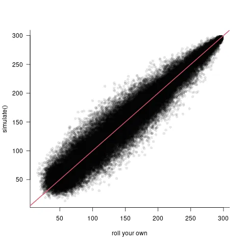
既然我无法通过simulate.merMod()完成我的目标,我决定尝试自己编写一个程序。问题在于,我需要确保这个程序是正确的。为了检查,我尝试将自己编写的结果与simulate.merMod()的结果进行比较(适当设置种子以使“随机”结果相同)。
基本上,我的自编程序过程包括使用线性预测器构建。
抱歉我的问题很长,但结构很复杂,我看不到缩短讨论的方法。
虽然这与我提出的问题无关,但我的最终目标是从拟合的模型中模拟新数据,但实验设计与数据集不同。更改涉及更改复制数(复制品是基础随机效应)和更改与每个观测值相关联的二项式试验的数量。最终目标是通过模拟来检查复制次数和二项式试验次数对估计某个(复杂)参数的精度产生的相对影响。
我正在使用lme4 R软件包进行工作。
我本来希望能够通过simulate.merMod()函数的“newdata”参数调整生成模拟数据的实验设计,但我无法使其正常工作。我可能误解了一些内容。我太慢并且太愚蠢,无法遵循simulate.merMod()的帮助文件。
既然我无法通过simulate.merMod()完成我的目标,我决定尝试自己编写一个程序。问题在于,我需要确保这个程序是正确的。为了检查,我尝试将自己编写的结果与simulate.merMod()的结果进行比较(适当设置种子以使“随机”结果相同)。
基本上,我的自编程序过程包括使用线性预测器构建。
* fitted fixed effect coefficients from the fitted model
* random effects simulated on the basis of the fitted
  random effects variances and covarances
我将线性预测器的逻辑函数作为概率,最后使用rbinom()来根据这些概率和所需的“大小”生成随机样本。
当模型中只有一个随机效应时,我得到了一致性,但是当有两个随机效应时,我无法得到一致性,也不知道自己做错了什么。
对于单一随机效应设置,我使用了lme4包中的“cbpp”数据集。 我使用的代码如下:
library(lme4)
fit   <- glmer(cbind(incidence, size - incidence) ~ 0 + period + (1 | herd),
             family = binomial, data = cbpp)
ccc   <- getME(fit,"beta")
sigma <- getME(fit,"theta")

# Roll-your-own:
set.seed(101)
Z     <- rnorm(length(levels(cbpp$herd)),0,sigma)
lnpr  <- with(cbpp,ccc[period] +  Z[herd])
p     <- 1/(1+exp(-lnpr))
s.ryo <- rbinom(nrow(cbpp),cbpp$size,p)

# Using simulate.merMod:
set.seed(101)
s.mer <- simulate(fit)
s.mer <- s.mer[,1][,1]

# Check for equality:
print(all.equal(s.ryo,s.mer))
这两个模拟结果完全一致。
然而,我真正感兴趣的场景涉及到两个随机效应(随机截距和随机“斜率”,即数值预测变量的随机系数)。接下来是我尝试在这种情况下使用的代码。在这种情况下,我无法让自己编写的代码和simulate.merMod()生成的结果一致。我在这种情况下使用的数据集不包含在lme4软件包中。这个数据集在说明性代码之后提供。
非常抱歉显示的内容相对较长。
我希望能得到任何关于我做错了什么的建议,并且希望得到关于我的自己编写的方法是否有意义的评论。
代码:
library(lme4)
fit   <- glmer(cbind(Good, Bad) ~ (trtmnt+0)/x + (x | batch),
               family = binomial, data = Dat) # See below for "Dat"
ccc   <- fixef(fit)
Sigma <- VarCorr(fit)[[1]]

# Roll-your-own:
set.seed(101)
nrep  <- length(levels(Dat$batch))
Z     <- MASS::mvrnorm(nrep,c(0,0),Sigma)
beta0 <- ccc[1:4][as.numeric(Dat$trtmnt)]
beta1 <- ccc[5:8][as.numeric(Dat$trtmnt)]
lnpr  <- with(Dat,beta0 + beta1*x + Z[batch,1] + Z[batch,2]*x)
p     <- 1/(1+exp(-lnpr)) # Inverse of logit link.
size  <- with(Dat,Good+Bad)
s.ryo <- rbinom(nrow(Dat),size,p)

# Using simulate.merMod:
set.seed(101)
s.mer <- simulate(fit)
s.mer <- s.mer[,1][,1]

# The results are not equal.
数据:
Dat <- structure(list(Good = c(87, 137, 194, 211, 250, 259, 272, 277,
279, 279, 279, 279, 76, 134, 216, 229, 253, 264, 275, 282, 286,
287, 287, 287, 90, 109, 209, 219, 228, 245, 240, 244, 247, 247,
247, 247, 113, 147, 230, 257, 283, 287, 290, 295, 298, 298, 298,
298, 60, 105, 175, 203, 237, 250, 263, 268, 267, 268, 268, 268,
32, 71, 163, 184, 206, 220, 231, 242, 243, 245, 245, 245, 104,
138, 254, 265, 261, 284, 282, 283, 285, 286, 286, 286, 57, 89,
155, 193, 210, 214, 219, 229, 231, 231, 231, 231, 42, 71, 136,
154, 197, 211, 226, 228, 229, 229, 229, 229, 47, 69, 140, 167,
208, 215, 235, 241, 244, 246, 246, 246, 49, 79, 138, 179, 198,
213, 214, 220, 220, 221, 221, 221, 57, 85, 170, 186, 224, 221,
231, 232, 234, 235, 235, 235, 57, 92, 162, 185, 219, 234, 240,
243, 242, 243, 243, 243, 55, 95, 178, 205, 237, 255, 263, 274,
274, 276, 278, 278, 53, 81, 183, 236, 243, 279, 285, 290, 288,
291, 291, 291, 72, 101, 166, 209, 223, 219, 238, 236, 238, 238,
238, 238, 49, 77, 135, 171, 182, 195, 205, 211, 213, 214, 214,
214, 214, 28, 63, 123, 144, 160, 182, 187, 198, 201, 203, 204,
205, 205, 36, 64, 169, 183, 190, 206, 211, 213, 216, 217, 218,
218, 218, 58, 76, 163, 182, 194, 198, 204, 203, 207, 207, 208,
208, 208, 41, 82, 145, 163, 195, 213, 221, 226, 228, 229, 229,
229, 229, 42, 66, 121, 153, 179, 187, 203, 214, 216, 216, 218,
218, 218, 57, 71, 132, 185, 190, 198, 205, 207, 209, 210, 210,
210, 210, 43, 68, 132, 174, 186, 190, 199, 206, 206, 208, 208,
208, 208, 38, 65, 115, 126, 178, 190, 203, 211, 212, 213, 213,
213, 213, 34, 66, 124, 144, 183, 199, 224, 227, 232, 234, 235,
235, 235, 37, 81, 132, 166, 182, 190, 212, 218, 218, 220, 220,
220, 220, 42, 73, 129, 180, 207, 214, 242, 245, 247, 247, 248,
248, 248), Bad = c(192, 142, 85, 68, 29, 20, 7, 2, 0, 0, 0, 0,
211, 153, 71, 58, 34, 23, 12, 5, 1, 0, 0, 0, 157, 138, 38, 28,
19, 2, 7, 3, 0, 0, 0, 0, 185, 151, 68, 41, 15, 11, 8, 3, 0, 0,
0, 0, 208, 163, 93, 65, 31, 18, 5, 0, 1, 0, 0, 0, 213, 174, 82,
61, 39, 25, 14, 3, 2, 0, 0, 0, 182, 148, 32, 21, 25, 2, 4, 3,
1, 0, 0, 0, 174, 142, 76, 38, 21, 17, 12, 2, 0, 0, 0, 0, 187,
158, 93, 75, 32, 18, 3, 1, 0, 0, 0, 0, 199, 177, 106, 79, 38,
31, 11, 5, 2, 0, 0, 0, 172, 142, 83, 42, 23, 8, 7, 1, 1, 0, 0,
0, 178, 150, 65, 49, 11, 14, 4, 3, 1, 0, 0, 0, 186, 151, 81,
58, 24, 9, 3, 0, 1, 0, 0, 0, 223, 183, 100, 73, 41, 23, 15, 4,
4, 2, 0, 0, 238, 210, 108, 55, 48, 12, 6, 1, 3, 0, 0, 0, 166,
137, 72, 29, 15, 19, 0, 2, 0, 0, 0, 0, 165, 137, 79, 43, 32,
19, 9, 3, 1, 0, 0, 0, 0, 177, 142, 82, 61, 45, 23, 18, 7, 4,
2, 1, 0, 0, 182, 154, 49, 35, 28, 12, 7, 5, 2, 1, 0, 0, 0, 150,
132, 45, 26, 14, 10, 4, 5, 1, 1, 0, 0, 0, 188, 147, 84, 66, 34,
16, 8, 3, 1, 0, 0, 0, 0, 176, 152, 97, 65, 39, 31, 15, 4, 2,
2, 0, 0, 0, 153, 139, 78, 25, 20, 12, 5, 3, 1, 0, 0, 0, 0, 165,
140, 76, 34, 22, 18, 9, 2, 2, 0, 0, 0, 0, 175, 148, 98, 87, 35,
23, 10, 2, 1, 0, 0, 0, 0, 201, 169, 111, 91, 52, 36, 11, 8, 3,
1, 0, 0, 0, 183, 139, 88, 54, 38, 30, 8, 2, 2, 0, 0, 0, 0, 206,
175, 119, 68, 41, 34, 6, 3, 1, 1, 0, 0, 0), x = c(1, 2, 3, 4,
5, 6, 7, 8, 9, 10, 12, 14, 1, 2, 3, 4, 5, 6, 7, 8, 9, 10, 12,
14, 1, 2, 3, 4, 5, 6, 7, 8, 9, 10, 12, 14, 1, 2, 3, 4, 5, 6,
7, 8, 9, 10, 12, 14, 1, 2, 3, 4, 5, 6, 7, 8, 9, 10, 12, 14, 1,
2, 3, 4, 5, 6, 7, 8, 9, 10, 12, 14, 1, 2, 3, 4, 5, 6, 7, 8, 9,
10, 12, 14, 1, 2, 3, 4, 5, 6, 7, 8, 9, 10, 12, 14, 1, 2, 3, 4,
5, 6, 7, 8, 9, 10, 12, 14, 16, 1, 2, 3, 4, 5, 6, 7, 8, 9, 10,
12, 14, 16, 1, 2, 3, 4, 5, 6, 7, 8, 9, 10, 12, 14, 16, 1, 2,
3, 4, 5, 6, 7, 8, 9, 10, 12, 14, 16, 1, 2, 3, 4, 5, 6, 7, 8,
9, 10, 12, 14, 16, 1, 2, 3, 4, 5, 6, 7, 8, 9, 10, 12, 14, 16,
1, 2, 3, 4, 5, 6, 7, 8, 9, 10, 12, 14, 16, 1, 2, 3, 4, 5, 6,
7, 8, 9, 10, 12, 14, 16, 1, 2, 3, 4, 5, 6, 7, 8, 9, 10, 12, 14,
16, 1, 2, 3, 4, 5, 6, 7, 8, 9, 10, 12, 14, 16, 1, 2, 3, 4, 5,
6, 7, 8, 9, 10, 12, 14, 16, 1, 2, 3, 4, 5, 6, 7, 8, 9, 10, 12,
14, 16), batch = structure(c(1L, 1L, 1L, 1L, 1L, 1L, 1L, 1L,
1L, 1L, 1L, 1L, 1L, 1L, 1L, 1L, 1L, 1L, 1L, 1L, 1L, 1L, 1L, 1L,
1L, 1L, 1L, 1L, 1L, 1L, 1L, 1L, 1L, 1L, 1L, 1L, 1L, 1L, 1L, 1L,
1L, 1L, 1L, 1L, 1L, 1L, 1L, 1L, 3L, 3L, 3L, 3L, 3L, 3L, 3L, 3L,
3L, 3L, 3L, 3L, 3L, 3L, 3L, 3L, 3L, 3L, 3L, 3L, 3L, 3L, 3L, 3L,
3L, 3L, 3L, 3L, 3L, 3L, 3L, 3L, 3L, 3L, 3L, 3L, 3L, 3L, 3L, 3L,
3L, 3L, 3L, 3L, 3L, 3L, 3L, 3L, 5L, 5L, 5L, 5L, 5L, 5L, 5L, 5L,
5L, 5L, 5L, 5L, 5L, 5L, 5L, 5L, 5L, 5L, 5L, 5L, 5L, 5L, 5L, 5L,
5L, 5L, 5L, 5L, 5L, 5L, 5L, 5L, 5L, 5L, 5L, 5L, 5L, 5L, 5L, 5L,
5L, 5L, 5L, 5L, 5L, 5L, 5L, 5L, 7L, 7L, 7L, 7L, 7L, 7L, 7L, 7L,
7L, 7L, 7L, 7L, 7L, 7L, 7L, 7L, 7L, 7L, 7L, 7L, 7L, 7L, 7L, 7L,
7L, 7L, 7L, 7L, 7L, 7L, 7L, 7L, 7L, 7L, 7L, 7L, 7L, 7L, 7L, 7L,
7L, 7L, 7L, 7L, 7L, 7L, 7L, 7L, 2L, 2L, 2L, 2L, 2L, 2L, 2L, 2L,
2L, 2L, 2L, 2L, 2L, 2L, 2L, 2L, 2L, 2L, 2L, 2L, 2L, 2L, 2L, 2L,
2L, 2L, 2L, 2L, 2L, 2L, 2L, 2L, 2L, 2L, 2L, 2L, 2L, 2L, 2L, 2L,
2L, 2L, 2L, 2L, 2L, 2L, 2L, 2L, 2L, 2L, 2L, 2L, 4L, 4L, 4L, 4L,
4L, 4L, 4L, 4L, 4L, 4L, 4L, 4L, 4L, 4L, 4L, 4L, 4L, 4L, 4L, 4L,
4L, 4L, 4L, 4L, 4L, 4L, 4L, 4L, 4L, 4L, 4L, 4L, 4L, 4L, 4L, 4L,
4L, 4L, 4L, 4L, 4L, 4L, 4L, 4L, 4L, 4L, 4L, 4L, 4L, 4L, 4L, 4L,
6L, 6L, 6L, 6L, 6L, 6L, 6L, 6L, 6L, 6L, 6L, 6L, 6L, 6L, 6L, 6L,
6L, 6L, 6L, 6L, 6L, 6L, 6L, 6L, 6L, 6L, 6L, 6L, 6L, 6L, 6L, 6L,
6L, 6L, 6L, 6L, 6L, 6L, 6L, 6L, 6L, 6L, 6L, 6L, 6L, 6L, 6L, 6L,
6L, 6L, 6L, 6L), levels = c("1", "2", "3", "4", "5", "6", "7"
), class = "factor"), trtmnt = structure(c(1L, 1L, 1L, 1L, 1L,
1L, 1L, 1L, 1L, 1L, 1L, 1L, 2L, 2L, 2L, 2L, 2L, 2L, 2L, 2L, 2L,
2L, 2L, 2L, 3L, 3L, 3L, 3L, 3L, 3L, 3L, 3L, 3L, 3L, 3L, 3L, 4L,
4L, 4L, 4L, 4L, 4L, 4L, 4L, 4L, 4L, 4L, 4L, 1L, 1L, 1L, 1L, 1L,
1L, 1L, 1L, 1L, 1L, 1L, 1L, 2L, 2L, 2L, 2L, 2L, 2L, 2L, 2L, 2L,
2L, 2L, 2L, 3L, 3L, 3L, 3L, 3L, 3L, 3L, 3L, 3L, 3L, 3L, 3L, 4L,
4L, 4L, 4L, 4L, 4L, 4L, 4L, 4L, 4L, 4L, 4L, 1L, 1L, 1L, 1L, 1L,
1L, 1L, 1L, 1L, 1L, 1L, 1L, 2L, 2L, 2L, 2L, 2L, 2L, 2L, 2L, 2L,
2L, 2L, 2L, 3L, 3L, 3L, 3L, 3L, 3L, 3L, 3L, 3L, 3L, 3L, 3L, 4L,
4L, 4L, 4L, 4L, 4L, 4L, 4L, 4L, 4L, 4L, 4L, 1L, 1L, 1L, 1L, 1L,
1L, 1L, 1L, 1L, 1L, 1L, 1L, 2L, 2L, 2L, 2L, 2L, 2L, 2L, 2L, 2L,
2L, 2L, 2L, 3L, 3L, 3L, 3L, 3L, 3L, 3L, 3L, 3L, 3L, 3L, 3L, 4L,
4L, 4L, 4L, 4L, 4L, 4L, 4L, 4L, 4L, 4L, 4L, 1L, 1L, 1L, 1L, 1L,
1L, 1L, 1L, 1L, 1L, 1L, 1L, 1L, 2L, 2L, 2L, 2L, 2L, 2L, 2L, 2L,
2L, 2L, 2L, 2L, 2L, 3L, 3L, 3L, 3L, 3L, 3L, 3L, 3L, 3L, 3L, 3L,
3L, 3L, 4L, 4L, 4L, 4L, 4L, 4L, 4L, 4L, 4L, 4L, 4L, 4L, 4L, 1L,
1L, 1L, 1L, 1L, 1L, 1L, 1L, 1L, 1L, 1L, 1L, 1L, 2L, 2L, 2L, 2L,
2L, 2L, 2L, 2L, 2L, 2L, 2L, 2L, 2L, 3L, 3L, 3L, 3L, 3L, 3L, 3L,
3L, 3L, 3L, 3L, 3L, 3L, 4L, 4L, 4L, 4L, 4L, 4L, 4L, 4L, 4L, 4L,
4L, 4L, 4L, 1L, 1L, 1L, 1L, 1L, 1L, 1L, 1L, 1L, 1L, 1L, 1L, 1L,
2L, 2L, 2L, 2L, 2L, 2L, 2L, 2L, 2L, 2L, 2L, 2L, 2L, 3L, 3L, 3L,
3L, 3L, 3L, 3L, 3L, 3L, 3L, 3L, 3L, 3L, 4L, 4L, 4L, 4L, 4L, 4L,
4L, 4L, 4L, 4L, 4L, 4L, 4L), levels = c("A", "B", "C", "D"), class = "factor")), row.names = c(NA,
348L), class = "data.frame")