将平均值合并在一起，不重复，并缩小最终数据框。

Question

将平均值合并在一起，不重复，并缩小最终数据框。

3

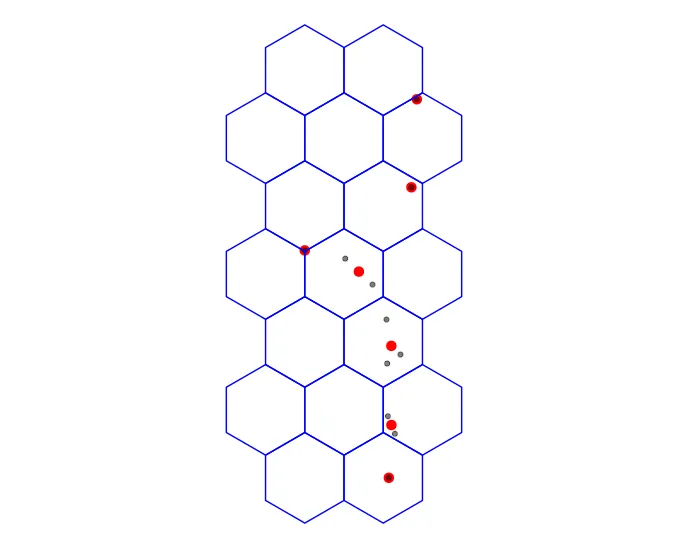
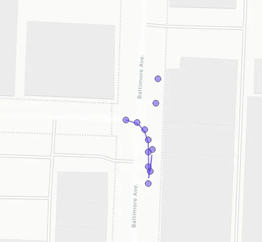
目标是在不重复任何点的情况下将10米内的点平均在一起，将点数据框减少到平均点，并理想地沿着收集这些点的路线获得点的平滑流动。这是一个来自较大文件（25,000次观察）的11点子集示例数据框：

library(sf)
df <- data.frame(trait = as.numeric(c(91.22,91.22,91.22,91.58,91.47,92.19,92.19,90.57,90.57,91.65,91.65)), 
                 datetime = as.POSIXct(c("2021-08-06 15:08:43","2021-08-06 15:08:44","2021-08-06 15:08:46","2021-08-06 15:08:47","2021-08-06 15:43:17","2021-08-06 15:43:18","2021-08-06 15:43:19","2021-08-06 15:43:20","2021-08-06 15:43:21","2021-08-06 15:43:22","2021-08-06 15:43:23")),
                 lat = c(39.09253, 39.09262, 39.09281, 39.09291, 39.09248, 39.09255, 39.09261, 39.09266, 39.0927, 39.09273, 39.09274),
                 lon = c(-94.58463, -94.58462, -94.5846, -94.58459, -94.58464, -94.58464, -94.58464, -94.58464, -94.58466, -94.5847, -94.58476)
                 ) # just to add some value that is plotable
projcrs <- "+proj=longlat +datum=WGS84 +no_defs +ellps=WGS84 +towgs84=0,0,0"
df <- st_as_sf(x = df,                         
               coords = c("lon", "lat"),
               crs = projcrs)

这是我尝试过的：

多次尝试使用st_is_within_distance(trav, trav, tolerance)，包括：
所展示的聚合方法。这些方法不起作用，因为同一点被多次平均。
通过尝试在lapply中动态更新列表来使用filter和across，但最终没有成功。
Jeffreyevans提供的这个帖子对我很有帮助，但并没有真正解决问题，而且有点过时了。
spThin包不起作用，因为它是针对更特定的变量设计的。
我想使用这个帖子进行聚类，但是聚类会产生随机点，实际上不能有效地减小数据框。

下面是我接近解决问题的方法。这种解决方法的问题在于在收集平均值时重复了点，这样会给某些点带来更多的权重。

  # first set tolerance
  tolerance <- 20 # 20 meters
  
  # get distance between points
  i <- st_is_within_distance(df, df, tolerance)
  
  # filter for indices with more than 1 (self) neighbor
  i <- i[which(lengths(i) > 1)]   
 
  # filter for unique indices (point 1, 2 / point 2, 1)
  i <- i[!duplicated(i)]
    
  # points in `sf` object that have no neighbors within tolerance
  no_neighbors <- trav[!(1:nrow(df) %in% unlist(i)),  ]  

  # iterate over indices of neighboring points
  avg_points <- lapply(i, function(b){
    df <- df[unlist(b), ]
    coords <- st_coordinates(df)
    
    df <- df %>%
      st_drop_geometry() %>%
      cbind(., coords)
    
    df_sum <-  df %>%
      summarise(
        datetime = first(datetime),
        trait = mean(trait),
        X = mean(X),
        Y = mean(Y),
        .groups = 'drop') %>% 
        ungroup()

    return(df)
  }) %>% 
    
    bind_rows() %>% 
    st_as_sf(coords = c('X', 'Y'),
             crs = "+proj=longlat +datum=WGS84 +no_defs ")

- estebangatillo

假设日期时间列在创建特征列的新平均值时不重要，这样做是否正确？您想要特征的空间平均值，而不是时间或时空平均值，对吗？ - mrhellmann

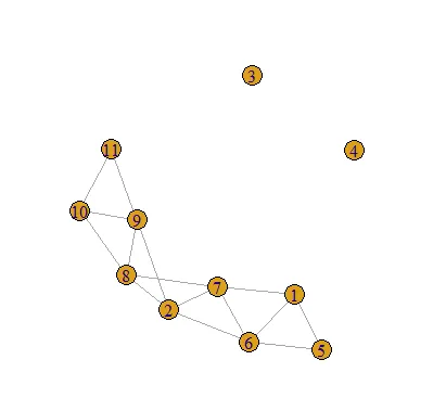
@mrhellmann 目前而言，我更感兴趣的是针对 trait 进行空间平均。我认为在 summarise 函数中将 datetime 变量设置为 first 是一种不错的方式，可以在不将其作为主要问题焦点的情况下进行包含。 - estebangatillo

只是为了澄清，当您说“不要在平均值中重复点”时，这是什么意思？在您的示例中，第1个和第2个点的相邻索引是1 2 5 6 7 8 9和1 2 5 6 7 8 9 10 11，这是否意味着对于第一个点，我们按照给定的平均值进行计算，但对于第二个点，仅在10和11之间（唯一尚未使用的索引）进行计算？如果是这种情况，那么对于没有剩余邻居的点会发生什么情况（甚至该点本身可能已经被包含在其他地方）？ - thothal

@thothal 是的！这正是我所想的。最初，没有邻居是使用以下方式选择的：no_neighbors <- trav[!(1:nrow(df) %in% unlist(i)), ]，然后它们被rbinded回来。 - estebangatillo

4个回答

0

如果目标是在聚类平均值中不给任何一个点更多的权重，那么使用加权平均值比尝试强制每个聚类包含一组与所有其他聚类不同的点更加平衡。

一种思考下面方法的方式是“切割”每个观察，并将这些碎片分配到聚类中，以使每个聚类中的碎片的权重总和为1。

这可能对于25k个观测来说太昂贵了，因此一个选项是在重叠或非重叠的段上执行此操作，然后将它们拼接在一起。

library(sf)
library(Rfast) # for the 'eachrow' function

df <- data.frame(trait = as.numeric(c(91.22,91.22,91.22,91.58,91.47,92.19,92.19,90.57,90.57,91.65,91.65)), 
                 datetime = as.POSIXct(c("2021-08-06 15:08:43","2021-08-06 15:08:44","2021-08-06 15:08:46","2021-08-06 15:08:47","2021-08-06 15:43:17","2021-08-06 15:43:18","2021-08-06 15:43:19","2021-08-06 15:43:20","2021-08-06 15:43:21","2021-08-06 15:43:22","2021-08-06 15:43:23")),
                 lat = c(39.09253, 39.09262, 39.09281, 39.09291, 39.09248, 39.09255, 39.09261, 39.09266, 39.0927, 39.09273, 39.09274),
                 lon = c(-94.58463, -94.58462, -94.5846, -94.58459, -94.58464, -94.58464, -94.58464, -94.58464, -94.58466, -94.5847, -94.58476)
) # just to add some value that is plotable
projcrs <- "+proj=longlat +datum=WGS84 +no_defs +ellps=WGS84 +towgs84=0,0,0"
df <- st_as_sf(x = df,                         
               coords = c("lon", "lat"),
               crs = projcrs)
n <- nrow(df)
# sum the trait column for a sanity check after calculations
sumtrait <- sum(df$trait)

# first set tolerance
tolerance <- 20 # 20 meters
tol <- 1e-5 # tolerance for the weight matrix marginal sums
# create clusters of points grouped by circles centered at each point
i <- st_is_within_distance(df, df, tolerance)
# Initialize a matrix for the weight of each point within each cluster. The
# initial value represents an unweighted average for each cluster, so the row
# sums are not necessarily 1.
sz <- lengths(i)
w <- replace(matrix(0, n, n), unlist(sapply(1:n, function(x) i[[x]] + n*(x - 1))), rep.int(1/sz, sz))
# iteratively adjust the weights until the marginal sums all equal 1 (within
# tolerance)
marg <- rowSums(w)

while (max(abs(marg - 1)) > tol) {
  w <- w/marg
  marg <- colSums(w)
  w <- eachrow(w, marg, "/")
  marg <- rowSums(w)
}

df$trait <- colSums(w*df$trait)
print(df, n = nrow(df))
#> Simple feature collection with 11 features and 2 fields
#> Geometry type: POINT
#> Dimension:     XY
#> Bounding box:  xmin: -94.58476 ymin: 39.09248 xmax: -94.58459 ymax: 39.09291
#> CRS:           +proj=longlat +datum=WGS84 +no_defs +ellps=WGS84 +towgs84=0,0,0
#>       trait            datetime                   geometry
#> 1  91.37719 2021-08-06 15:08:43 POINT (-94.58463 39.09253)
#> 2  91.44430 2021-08-06 15:08:44 POINT (-94.58462 39.09262)
#> 3  91.31374 2021-08-06 15:08:46  POINT (-94.5846 39.09281)
#> 4  91.46755 2021-08-06 15:08:47 POINT (-94.58459 39.09291)
#> 5  91.64053 2021-08-06 15:43:17 POINT (-94.58464 39.09248)
#> 6  91.37719 2021-08-06 15:43:18 POINT (-94.58464 39.09255)
#> 7  91.44430 2021-08-06 15:43:19 POINT (-94.58464 39.09261)
#> 8  91.41380 2021-08-06 15:43:20 POINT (-94.58464 39.09266)
#> 9  91.41380 2021-08-06 15:43:21  POINT (-94.58466 39.0927)
#> 10 91.31880 2021-08-06 15:43:22  POINT (-94.5847 39.09273)
#> 11 91.31880 2021-08-06 15:43:23 POINT (-94.58476 39.09274)

# check that the sum of the "traits" column is unchanged
sum(df$trait) - sumtrait
#> [1] 4.875536e-07

更新：如果确实需要一种独占式分组方法，那么可以采用贪心算法来实现：

avg_points <- numeric(nrow(df))
clusters <- vector("list", nrow(df))
currclust <- 0L
df$unused <- TRUE
for (cl in seq_along(df)) {
  if (sum(df$unused[i[[cl]]])) {
    currclust <- currclust + 1L
    avg_points[currclust] <- mean(df$trait[i[[cl]]][df$unused[i[[cl]]]])
    clusters[[currclust]] <- i[[cl]][df$unused[i[[cl]]]]
    df$unused[i[[cl]]] <- FALSE
  }
}

avg_points <- avg_points[1:currclust]
clusters <- clusters[1:currclust]
avg_points
#> [1] 91.34714 91.65000 91.40000
clusters
#> [[1]]
#> [1] 1 2 5 6 7 8 9
#> 
#> [[2]]
#> [1] 10 11
#> 
#> [[3]]
#> [1] 3 4

请注意，不均匀加权的问题仍然存在 - 第1组中的观测值每个加权为1/7，而第2组和第3组中的观测值每个加权为1/2。

- jblood94

谢谢！由于while()函数中的eachrow()函数，我无法运行它...这是什么？我以前从未见过。另外，我更新了我的问题，澄清我正在尝试将完整数据框减少到只有平均值。例如，我可能只有6个点，而不是11个。 - estebangatillo

它在Rfast包中，因此我的代码顶部需要加上library(Rfast)。 - jblood94

哦，天哪。我早上不是一个有精神的人。我运行了 install.packages 但忘记添加库了。真是自己给自己打脸啊。谢谢！ - estebangatillo

关于数据减少，请参见我原始答案下面的更新。 - jblood94

0

我不确定，但也许这就是您正在寻找的内容？

您可以尝试使用smoothr::smooth()的不同设置/方法来获得所需的结果。

library(tidyverse)
library(igraph)
library(smoothr)
library(mapview)  # for viewing purposes only
# get a matrix of points <10 meter apart
m <- st_is_within_distance(df, dist = 10, sparse = FALSE)
# creata an igraph from the matrix
g <- graph.adjacency(m, mode="undirected", diag = FALSE)
plot(g)

彼此之间距离在10米以内的点？

# pass cluster-number to df object
df$id <- as.vector(components(G)$membership)
# create polylines (only if more than 1 point!)
df.lines <- df %>%
  group_by(id) %>%
  dplyr::add_tally() %>%
  dplyr::filter(n > 1) %>%
  summarise(geometry = st_combine(geometry)) %>%
  st_cast("LINESTRING") %>%
  # create smooth lines
  smoothr::smooth(method = "ksmooth")
#view points and lines
mapview::mapview(list(df, df.lines))

- Wimpel

0

如果我正确理解了您的问题，那么所有问题都归结为选择“正确”的邻居，即那些在某个邻域内且尚未使用过的邻居。如果没有这样的邻居，则仅使用该点本身（即使它已经在另一个点的平均值计算中使用过）。

以下是使用purrr :: accumulate解决方案，首先生成正确的索引，然后仅使用这些索引进行平均：

library(purrr)
library(dplyr)

idx <- accumulate(i[-1L], function(x, y) {
   x$points <- setdiff(y, x$used)
   x$used <- union(x$used, y)
   x
}, .init = list(used = i[[1L]], points = i[[1L]]))

idx[1:4]

# [[1]]
# [[1]]$used
# [1] 1 2 5 6 7 8 9
# 
# [[1]]$points
# [1] 1 2 5 6 7 8 9
#
# 
# [[2]]
# [[2]]$used
# [1]  1  2  5  6  7  8  9 10 11
# 
# [[2]]$points
# [1] 10 11
#
#
# [[3]]
# [[3]]$used
# [1]  1  2  5  6  7  8  9 10 11  3  4
# 
# [[3]]$points
# [1] 3 4
#
#
# [[4]]
# [[4]]$used
# [1]  1  2  5  6  7  8  9 10 11  3  4
#
# [[4]]$points
# integer(0)

想法是我们维护一个已使用索引的列表，即在任何邻域中已经使用的索引以及剩余项 (points)。例如，对于第一个点，我们使用索引为1,2,5,6,7,8,9的点，这仅留下索引为10,11的第二个点。如果没有点剩下，我们返回integer(0)。

现在，我们已经设置好了索引列表，其余的工作很容易，通过循环遍历列表，选择指定的点(如果没有点剩余，则使用点本身)，然后进行平均化。

idx %>% 
   imap_dfr(function(x, y) {
      if (!length(x$points)) {
         idx <- y
      } else {
         idx <- x$points
      }
      df[idx, , drop = FALSE] %>% 
         bind_cols(st_coordinates(.) %>% as_tibble()) %>% 
         st_drop_geometry() %>% 
         summarise(datetime = first(datetime),
                   trait = mean(trait),
                   X = mean(X),
                   Y = mean(Y))
   }) %>% 
   st_as_sf(coords = c('X', 'Y'),
            crs = "+proj=longlat +datum=WGS84 +no_defs ") 

# Simple feature collection with 11 features and 2 fields
# Geometry type: POINT
# Dimension:     XY
# Bounding box:  xmin: -94.58476 ymin: 39.09248 xmax: -94.58459 ymax: 39.09291
# CRS:           +proj=longlat +datum=WGS84 +no_defs 
# First 10 features:
#               datetime    trait                   geometry
# 1  2021-08-06 15:08:43 91.34714 POINT (-94.58464 39.09259)
# 2  2021-08-06 15:43:22 91.65000 POINT (-94.58473 39.09274)
# 3  2021-08-06 15:08:46 91.40000  POINT (-94.5846 39.09286)
# 4  2021-08-06 15:08:47 91.58000 POINT (-94.58459 39.09291)
# 5  2021-08-06 15:43:17 91.47000 POINT (-94.58464 39.09248)
# 6  2021-08-06 15:43:18 92.19000 POINT (-94.58464 39.09255)
# 7  2021-08-06 15:43:19 92.19000 POINT (-94.58464 39.09261)
# 8  2021-08-06 15:43:20 90.57000 POINT (-94.58464 39.09266)
# 9  2021-08-06 15:43:21 90.57000  POINT (-94.58466 39.0927)
# 10 2021-08-06 15:43:22 91.65000  POINT (-94.5847 39.09273)

- thothal

网页内容由stack overflow 提供, 点击上面的

可以查看英文原文，
原文链接

- mrhellmann · Accepted Answer

另一个答案使用sf::aggregate()和六边形网格来找到彼此距离在特定范围内的点。也可以使用正方形网格。结果会因网格与点的相对位置而有所不同，但每个点都不应在确定平均值时重复使用。

步骤概述：

加载数据，将其转换为CRS 5070以进行米制测量
获取数据的边界框
创建一个由每个直径约为10米的边界框组成的六边形网格
使用mean聚合落在同一六边形中的点
将其连接到原始数据

library(sf)
library(tidyverse)

set.seed(22) # might be needed to get same hex grid?

#### your sample data
df <- data.frame(trait = as.numeric(c(91.22,91.22,91.22,91.58,91.47,92.19,92.19,90.57,90.57,91.65,91.65)), 
                 datetime = as.POSIXct(c("2021-08-06 15:08:43","2021-08-06 15:08:44","2021-08-06 15:08:46","2021-08-06 15:08:47","2021-08-06 15:43:17","2021-08-06 15:43:18","2021-08-06 15:43:19","2021-08-06 15:43:20","2021-08-06 15:43:21","2021-08-06 15:43:22","2021-08-06 15:43:23")),
                 lat = c(39.09253, 39.09262, 39.09281, 39.09291, 39.09248, 39.09255, 39.09261, 39.09266, 39.0927, 39.09273, 39.09274),
                 lon = c(-94.58463, -94.58462, -94.5846, -94.58459, -94.58464, -94.58464, -94.58464, -94.58464, -94.58466, -94.5847, -94.58476)
) # just to add some value that is plotable
projcrs <- "+proj=longlat +datum=WGS84 +no_defs +ellps=WGS84 +towgs84=0,0,0"
df <- st_as_sf(x = df,                         
               coords = c("lon", "lat"),
               crs = projcrs) %>%
  st_transform(5070)  ### transform to 5070 for a projection in meters
#### end sample data


# Get a bounding box as an sf object to make a grid
bbox <- st_bbox(df) %>% st_as_sfc()

# Make a grid as hexagons with approximately the right size 
#  area ~86m; side ~5.75m; long diag ~11.5m 
hex_grid <- st_make_grid(bbox, cellsize = 10, square = F) %>% st_as_sf()

# Aggregate mean of the hexagonal grid
hex_agg <- aggregate(df ,
                     hex_grid,
                     mean,
                     join = st_contains) %>% filter(!is.na(trait))

# Assign the mean of the hexagon to points that fall 
#  within each hexagon
df_agg <- st_join(df, hex_agg)

head(df_agg) # trait.x from df, trait.y from the mean by hexagon
#> Simple feature collection with 6 features and 4 fields
#> Geometry type: POINT
#> Dimension:     XY
#> Bounding box:  xmin: 121281.6 ymin: 1786179 xmax: 121285.3 ymax: 1786227
#> Projected CRS: NAD83 / Conus Albers
#>   trait.x          datetime.x  trait.y          datetime.y
#> 1   91.22 2021-08-06 15:08:43 91.70500 2021-08-06 15:26:00
#> 2   91.22 2021-08-06 15:08:44 91.32667 2021-08-06 15:31:47
#> 3   91.22 2021-08-06 15:08:46 91.22000 2021-08-06 15:08:46
#> 4   91.58 2021-08-06 15:08:47 91.58000 2021-08-06 15:08:47
#> 5   91.47 2021-08-06 15:43:17 91.47000 2021-08-06 15:43:17
#> 6   92.19 2021-08-06 15:43:18 91.70500 2021-08-06 15:26:00
#>                   geometry
#> 1 POINT (121282.5 1786184)
#> 2 POINT (121283.2 1786194)
#> 3 POINT (121284.6 1786216)
#> 4 POINT (121285.3 1786227)
#> 5 POINT (121281.7 1786179)
#> 6 POINT (121281.6 1786186)

sum(df_agg$trait.x) - sum(df_agg$trait.y) # original trait - aggregate trait should be 0, or near 0
#> [1] 0

ggplot(df_agg) + 
  geom_sf(aes(size = trait.x), alpha = .2, color = 'blue') +  # Original triat
  geom_sf(aes(size = trait.y), alpha = .2, color = 'red') +  # New aggregated trait
  theme_void()

按特征大小分类。蓝点是原始数据，红色是新的空间平均值。


## Plot of
# original points & hex grid used:
ggplot() + 
  geom_sf(data = df, color = 'red') + 
  geom_sf(data = hex_grid, fill = NA) +
  theme_void()

图表显示了平均值的点分组情况。看起来每个六边形的平均值有1、2和3个点的分组。

^{由reprex package（v2.0.1）于2022年3月23日创建}

编辑

更新为每个六边形仅有一个点，损失了部分原始点

## Edit for one point per hexagon:
hex_agg <- aggregate(df ,
                     hex_grid,
                     mean,
                     join = st_contains) %>% filter(!is.na(trait)) %>%
  rownames_to_column('hex_num')  # add hexagon number to group_by

## Guide to join on, has only hexagon number & centroid of contained points
hex_guide <- df_agg %>%
  group_by(hex_num) %>%
  summarise() %>%
  st_centroid()

# The full sf object with only one point per hexagon
#  this join isn't the most efficient, but slice(1) removes
#  the duplicate data. You could clean df_agg before the join
#  to resolve this
final_join <- df_agg %>%
                 st_drop_geometry() %>%
                 left_join(hex_guide, by = 'hex_num') %>% 
                 group_by(hex_num) %>%
                 slice(1) %>%
                 ungroup() %>%
                 st_as_sf()

ggplot() +
  geom_sf(data = final_join, color = 'red', size = 3) +
  geom_sf(data = df, color = 'black', alpha = .5) +
  geom_sf(data = hex_grid, color = 'blue', fill = NA)

该图显示了六边形，原始数据点为灰色，新的红色点位于分组原始点的质心。每个六边形只有一个红点。