这个波形相当简单,因此我们将拟合一个多项式曲线到由cv2输出定义的主要边缘。首先,我们想要获取该主要边缘的点。假设您的原点在图像上是左上角。查看原始图像,如果我们只取范围在(750,1500)之间具有最大y的点,那么我们对感兴趣的点会有一个很好的近似。
import cv2
import numpy as np
from matplotlib import pyplot as plt
from numba import jit
img = cv2.imread('wave.jpg',0)
edges = cv2.Canny(img,100,200)
@jit(nopython=True)
def find_first(item, vec):
"""return the index of the first occurence of item in vec"""
for i in range(len(vec)):
if item == vec[i]:
return i
return -1
bounds = [750, 1500]
window = edges[bounds[1]:bounds[0]:-1].transpose()
xy = []
for i in range(len(window)):
col = window[i]
j = find_first(255, col)
if j != -1:
xy.extend((i, j))
data = np.array(xy).reshape((-1, 2))
data[:, 1] = bounds[1] - data[:, 1]
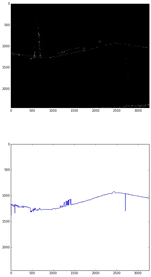
如果我们将这些点绘制成图表,就可以看到它们非常接近我们的目标点。
plt.figure(1, figsize=(8, 16))
ax1 = plt.subplot(211)
ax1.imshow(edges,cmap = 'gray')
ax2 = plt.subplot(212)
ax2.axis([0, edges.shape[1], edges.shape[0], 0])
ax2.plot(data[:,1])
plt.show()
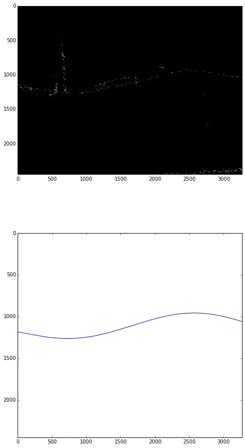
现在我们有了一个坐标对的数组,我们可以使用numpy.polyfit生成最佳拟合曲线的系数,然后使用numpy.poly1d从这些系数生成函数。
xdata = data[:,0]
ydata = data[:,1]

z = np.polyfit(xdata, ydata, 5)
f = np.poly1d(z)
然后绘制图形以验证
t = np.arange(0, edges.shape[1], 1)
plt.figure(2, figsize=(8, 16))
ax1 = plt.subplot(211)
ax1.imshow(edges,cmap = 'gray')
ax2 = plt.subplot(212)
ax2.axis([0, edges.shape[1], edges.shape[0], 0])
ax2.plot(t, f(t))
plt.show()
 以下是边缘检测的结果:
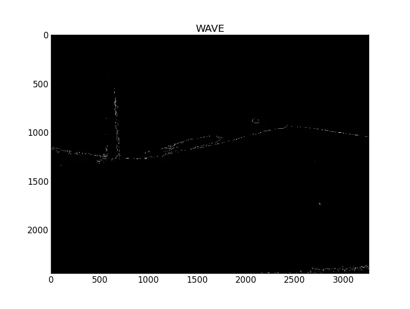 此代码是从OpenCV教程中的示例复制的。
numba只是为了通过编译使find_first操作更加高效而需要的。您可以删除导入语句和装饰器@jit(nopython=True)。我刚刚进行了一次测试,使用numba运行时间约为 80ms,而不使用它则需要约 3.5s,这是相当显著的,但根据您的应用程序仍然是合理的。 - Chris Hunt