我正在尝试在Python中实现一个Reed-Solomon编码器-解码器,支持纠删码的解码,但这让我感到非常困惑。
目前的实现只支持解码错误或擦除,但不能同时支持两者(即使它低于2*错误+擦除的理论界限)。
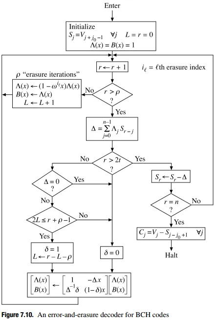
从Blahut的论文(此处和此处)中看来,我们只需要使用擦除定位多项式初始化错误定位多项式,就可以隐式地在Berlekamp-Massey中计算出纠正位置多项式。
这种方法对我来说部分有效:当2*errors+erasures < (n-k)/2时,它可以使用,但实际上在调试后只是因为BM计算一个错误定位多项式,该多项式得到与擦除定位多项式完全相同的值(因为我们低于仅纠错的误差限制),因此通过伽罗华域截短,我们最终获得了正确的擦除定位多项式的值(至少我是这样理解的,我可能是错的)。
然而,当我们超过(n-k)/2时,例如如果n=20且k=11,则我们有(n-k)=9个擦除的符号可以纠正,如果我们输入5个擦除,则BM就会出现问题。如果我们输入4个擦除+1个错误(由于我们仍然远低于界限,因为2*errors+erasures = 2+4 = 6 < 9),BM仍然会出现问题。
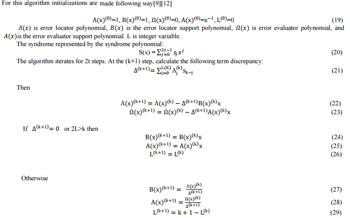
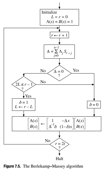
我实现的Berlekamp-Massey算法的确切算法可以在此演示文稿(第15-17页)中找到,但非常类似的描述可以在这里和这里找到,并在此处附上数学描述的副本:
Polynomial和GF256int分别是多项式和2^8上的伽罗瓦域的通用实现。这些类已经过单元测试,通常是无缺陷的。Reed-Solomon编码/解码方法的其余部分(例如Forney和Chien搜索)也是如此。这里有一个快速测试案例的完整代码:http://codepad.org/l2Qi0y8o。
以下是示例输出:
在这里,擦除解码总是正确的,因为它根本不使用BM来计算擦除定位器。通常,另外两个测试用例应该输出相同的sigma,但它们却没有。
目前的实现只支持解码错误或擦除,但不能同时支持两者(即使它低于2*错误+擦除的理论界限)。
从Blahut的论文(此处和此处)中看来,我们只需要使用擦除定位多项式初始化错误定位多项式,就可以隐式地在Berlekamp-Massey中计算出纠正位置多项式。
这种方法对我来说部分有效:当2*errors+erasures < (n-k)/2时,它可以使用,但实际上在调试后只是因为BM计算一个错误定位多项式,该多项式得到与擦除定位多项式完全相同的值(因为我们低于仅纠错的误差限制),因此通过伽罗华域截短,我们最终获得了正确的擦除定位多项式的值(至少我是这样理解的,我可能是错的)。
然而,当我们超过(n-k)/2时,例如如果n=20且k=11,则我们有(n-k)=9个擦除的符号可以纠正,如果我们输入5个擦除,则BM就会出现问题。如果我们输入4个擦除+1个错误(由于我们仍然远低于界限,因为2*errors+erasures = 2+4 = 6 < 9),BM仍然会出现问题。
我实现的Berlekamp-Massey算法的确切算法可以在此演示文稿(第15-17页)中找到,但非常类似的描述可以在这里和这里找到,并在此处附上数学描述的副本:
def _berlekamp_massey(self, s, k=None, erasures_loc=None):
    '''Computes and returns the error locator polynomial (sigma) and the
    error evaluator polynomial (omega).
    If the erasures locator is specified, we will return an errors-and-erasures locator polynomial and an errors-and-erasures evaluator polynomial.
    The parameter s is the syndrome polynomial (syndromes encoded in a
    generator function) as returned by _syndromes. Don't be confused with
    the other s = (n-k)/2

    Notes:
    The error polynomial:
    E(x) = E_0 + E_1 x + ... + E_(n-1) x^(n-1)

    j_1, j_2, ..., j_s are the error positions. (There are at most s
    errors)

    Error location X_i is defined: X_i = a^(j_i)
    that is, the power of a corresponding to the error location

    Error magnitude Y_i is defined: E_(j_i)
    that is, the coefficient in the error polynomial at position j_i

    Error locator polynomial:
    sigma(z) = Product( 1 - X_i * z, i=1..s )
    roots are the reciprocals of the error locations
    ( 1/X_1, 1/X_2, ...)

    Error evaluator polynomial omega(z) is here computed at the same time as sigma, but it can also be constructed afterwards using the syndrome and sigma (see _find_error_evaluator() method).
    '''
    # For errors-and-erasures decoding, see: Blahut, Richard E. "Transform techniques for error control codes." IBM Journal of Research and development 23.3 (1979): 299-315. http://citeseerx.ist.psu.edu/viewdoc/download?doi=10.1.1.92.600&rep=rep1&type=pdf and also a MatLab implementation here: http://www.mathworks.com/matlabcentral/fileexchange/23567-reed-solomon-errors-and-erasures-decoder/content//RS_E_E_DEC.m
    # also see: Blahut, Richard E. "A universal Reed-Solomon decoder." IBM Journal of Research and Development 28.2 (1984): 150-158. http://citeseerx.ist.psu.edu/viewdoc/download?doi=10.1.1.84.2084&rep=rep1&type=pdf
    # or alternatively see the reference book by Blahut: Blahut, Richard E. Theory and practice of error control codes. Addison-Wesley, 1983.
    # and another good alternative book with concrete programming examples: Jiang, Yuan. A practical guide to error-control coding using Matlab. Artech House, 2010.
    n = self.n
    if not k: k = self.k

    # Initialize:
    if erasures_loc:
        sigma = [ Polynomial(erasures_loc.coefficients) ] # copy erasures_loc by creating a new Polynomial
        B = [ Polynomial(erasures_loc.coefficients) ]
    else:
        sigma =  [ Polynomial([GF256int(1)]) ] # error locator polynomial. Also called Lambda in other notations.
        B =    [ Polynomial([GF256int(1)]) ] # this is the error locator support/secondary polynomial, which is a funky way to say that it's just a temporary variable that will help us construct sigma, the error locator polynomial
    omega =  [ Polynomial([GF256int(1)]) ] # error evaluator polynomial. We don't need to initialize it with erasures_loc, it will still work, because Delta is computed using sigma, which itself is correctly initialized with erasures if needed.
    A =  [ Polynomial([GF256int(0)]) ] # this is the error evaluator support/secondary polynomial, to help us construct omega
    L =      [ 0 ] # necessary variable to check bounds (to avoid wrongly eliminating the higher order terms). For more infos, see https://www.cs.duke.edu/courses/spring11/cps296.3/decoding_rs.pdf
    M =      [ 0 ] # optional variable to check bounds (so that we do not mistakenly overwrite the higher order terms). This is not necessary, it's only an additional safe check. For more infos, see the presentation decoding_rs.pdf by Andrew Brown in the doc folder.

    # Polynomial constants:
    ONE = Polynomial(z0=GF256int(1))
    ZERO = Polynomial(z0=GF256int(0))
    Z = Polynomial(z1=GF256int(1)) # used to shift polynomials, simply multiply your poly * Z to shift

    s2 = ONE + s

    # Iteratively compute the polynomials 2s times. The last ones will be
    # correct
    for l in xrange(0, n-k):
        K = l+1
        # Goal for each iteration: Compute sigma[K] and omega[K] such that
        # (1 + s)*sigma[l] == omega[l] in mod z^(K)

        # For this particular loop iteration, we have sigma[l] and omega[l],
        # and are computing sigma[K] and omega[K]

        # First find Delta, the non-zero coefficient of z^(K) in
        # (1 + s) * sigma[l]
        # This delta is valid for l (this iteration) only
        Delta = ( s2 * sigma[l] ).get_coefficient(l+1) # Delta is also known as the Discrepancy, and is always a scalar (not a polynomial).
        # Make it a polynomial of degree 0, just for ease of computation with polynomials sigma and omega.
        Delta = Polynomial(x0=Delta)

        # Can now compute sigma[K] and omega[K] from
        # sigma[l], omega[l], B[l], A[l], and Delta
        sigma.append( sigma[l] - Delta * Z * B[l] )
        omega.append( omega[l] - Delta * Z * A[l] )

        # Now compute the next B and A
        # There are two ways to do this
        # This is based on a messy case analysis on the degrees of the four polynomials sigma, omega, A and B in order to minimize the degrees of A and B. For more infos, see https://www.cs.duke.edu/courses/spring10/cps296.3/decoding_rs_scribe.pdf
        # In fact it ensures that the degree of the final polynomials aren't too large.
        if Delta == ZERO or 2*L[l] > K \
            or (2*L[l] == K and M[l] == 0):
            # Rule A
            B.append( Z * B[l] )
            A.append( Z * A[l] )
            L.append( L[l] )
            M.append( M[l] )

        elif (Delta != ZERO and 2*L[l] < K) \
            or (2*L[l] == K and M[l] != 0):
            # Rule B
            B.append( sigma[l] // Delta )
            A.append( omega[l] // Delta )
            L.append( K - L[l] )
            M.append( 1 - M[l] )

        else:
            raise Exception("Code shouldn't have gotten here")

    return sigma[-1], omega[-1]
Polynomial和GF256int分别是多项式和2^8上的伽罗瓦域的通用实现。这些类已经过单元测试,通常是无缺陷的。Reed-Solomon编码/解码方法的其余部分(例如Forney和Chien搜索)也是如此。这里有一个快速测试案例的完整代码:http://codepad.org/l2Qi0y8o。
以下是示例输出:
Encoded message:
hello world�ꐙ�Ī`>
-------
Erasures decoding:
Erasure locator: 189x^5 + 88x^4 + 222x^3 + 33x^2 + 251x + 1
Syndrome: 149x^9 + 113x^8 + 29x^7 + 231x^6 + 210x^5 + 150x^4 + 192x^3 + 11x^2 + 41x
Sigma: 189x^5 + 88x^4 + 222x^3 + 33x^2 + 251x + 1
Symbols positions that were corrected: [19, 18, 17, 16, 15]
('Decoded message: ', 'hello world', '\xce\xea\x90\x99\x8d\xc4\xaa`>')
Correctly decoded:  True
-------
Errors+Erasures decoding for the message with only erasures:
Erasure locator: 189x^5 + 88x^4 + 222x^3 + 33x^2 + 251x + 1
Syndrome: 149x^9 + 113x^8 + 29x^7 + 231x^6 + 210x^5 + 150x^4 + 192x^3 + 11x^2 + 41x
Sigma: 101x^10 + 139x^9 + 5x^8 + 14x^7 + 180x^6 + 148x^5 + 126x^4 + 135x^3 + 68x^2 + 155x + 1
Symbols positions that were corrected: [187, 141, 90, 19, 18, 17, 16, 15]
('Decoded message: ', '\xf4\x00\x00\x00\x00\x00\x00\x00\x00\x00\x00\x00\x00\x00\x00\x00\x00\x00\x00\x00\x00\x00\x00\x00\x00\x00\x00\x00\x00\x00\x00\x00\x00\x00\x00\x00\x00\x00\x00\x00\x00\x00\x00\x00\x00\x00.\x00\x00\x00\x00\x00\x00\x00\x00\x00\x00\x00\x00\x00\x00\x00\x00\x00\x00\x00\x00\x00\x00\x00\x00\x00\x00\x00\x00\x00\x00\x00\x00\x00\x00\x00\x00\x00\x00\x00\x00\x00\x00\x00\x00\x00\x00\x00\x00\x00\x00P\x00\x00\x00\x00\x00\x00\x00\x00\x00\x00\x00\x00\x00\x00\x00\x00\x00\x00\x00\x00\x00\x00\x00\x00\x00\x00\x00\x00\x00\x00\x00\x00\x00\x00\x00\x00\x00\x00\x00\x00\x00\x00\x00\x00\x00\x00\x00\x00\x00\x00\x00\x00\x00\x00\x00\x00\x00\x00\x00\x00\x00\x00\x00\x00\x00\x00\x00\x00\x00\x00\xe3\xe6\xffO> world', '\xce\xea\x90\x99\x8d\xc4\xaa`>')
Correctly decoded:  False
-------
Errors+Erasures decoding for the message with erasures and one error:
Erasure locator: 77x^4 + 96x^3 + 6x^2 + 206x + 1
Syndrome: 49x^9 + 107x^8 + x^7 + 109x^6 + 236x^5 + 15x^4 + 8x^3 + 133x^2 + 243x
Sigma: 38x^9 + 98x^8 + 239x^7 + 85x^6 + 32x^5 + 168x^4 + 92x^3 + 225x^2 + 22x + 1
Symbols positions that were corrected: [19, 18, 17, 16]
('Decoded message: ', "\xda\xe1'\xccA world", '\xce\xea\x90\x99\x8d\xc4\xaa`>')
Correctly decoded:  False
在这里,擦除解码总是正确的,因为它根本不使用BM来计算擦除定位器。通常,另外两个测试用例应该输出相同的sigma,但它们却没有。
当你比较前两个测试用例时,问题来自于BM是显而易见的:综合症和擦除定位器是相同的,但结果sigma完全不同(在第二个测试中使用了BM,而在只有擦除的第一个测试用例中没有调用BM)。
非常感谢您的任何帮助或任何关于如何调试此问题的想法。请注意,您的答案可以是数学或代码,但请解释我的方法出了什么问题。
/编辑:仍然没有找到如何正确实现勘误BM解码器的方法(请参见下面的答案)。将奖励提供给能够解决问题(或至少指导我解决问题)的人。
/编辑2:我真傻,抱歉,我刚刚重新阅读了模式,并发现我错过了赋值L = r - L - erasures_count的更改... 我已经更新了代码以修复并重新接受了我的答案。
l不是一个好的变量名,因为它与1相似。i通常用作循环计数器。 - Craig McQueen