添加坐标轴标题后停止ggplots的大小重新调整

Question

添加坐标轴标题后停止ggplots的大小重新调整

4

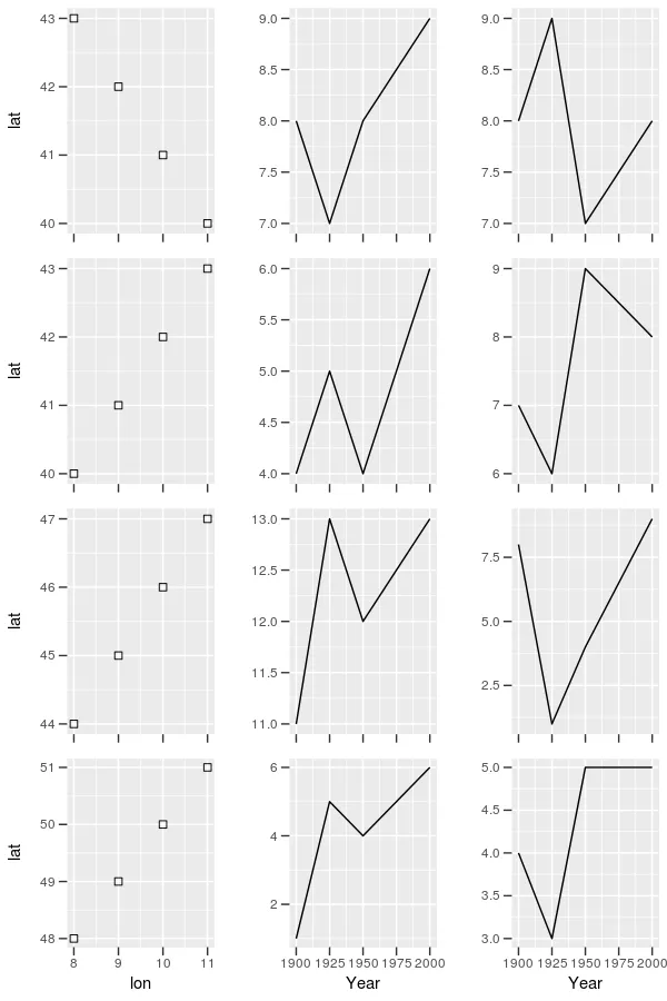
我有一个具有4x3面板结构的ggplot2。每列面板共享相同的x轴文本和标题。我希望所有面板的大小相同，但是当我将x轴标题和文本添加到底部行时，会导致面板重新调整大小。如何确保面板大小相等？以下是可重现的示例：

library(ggmap)
library(maps)
library(ggplot2)

BII.TEMP.SUMMER=data.frame("Year"=c(1851, 1901, 1951, 2001), "Temp"=c(8,7,8,9))
BII.PPT.SUMMER=data.frame("Year"=c(1851, 1901, 1951, 2001), "PPT"=c(8,7,8,9))
SCAN.TEMP.SUMMER=data.frame("Year"=c(1851, 1901, 1951, 2001), "Temp"=c(8,7,8,9))
SCAN.PPT.SUMMER=data.frame("Year"=c(1851, 1901, 1951, 2001), "PPT"=c(8,7,8,9))
CE.TEMP.SUMMER=data.frame("Year"=c(1851, 1901, 1951, 2001), "Temp"=c(8,7,8,9))
CE.PPT.SUMMER=data.frame("Year"=c(1851, 1901, 1951, 2001), "PPT"=c(8,7,8,9))
TEMP.SUMMER=data.frame("Year"=c(1851, 1901, 1951, 2001), "Temp"=c(8,7,8,9))
PPT.SUMMER=data.frame("Year"=c(1851, 1901, 1951, 2001), "PPT"=c(8,7,8,9))



BII.coords=data.frame(lon=c(-6.9532,-7.9925,-2.5036,-8.2569,-6.5487,-7.4083,-2.0369,-2.175,-6.1921), 
                          lat=c(53.3653,53.0807,55.0875,53.1865,54.8862,53.7667,54.4253,54.0964,55.0848))

CE.coords=data.frame(lon=c(16.5872,13.8494,6.2317,21.2201,15.3602,17.9821,18.3098,
                           9.8544,22.4419,6.1736,16.4785,18.0833,24.545), 
                     lat=c(53.8078,53.0558,46.5397,53.8726,50.8519,53.5918,53.188,
                           46.49,54.3314,46.5667,54.3619,54.4244,47.5739))

SCAN.coords=data.frame(lon=c(17.3667,18.6833,18.4333,22.7833,19.5828,10.1896,26.25,19.0484), 
                       lat=c(60.0167,59.9667,59.6333,60.7833,64.1647,56.8391,58.8667,68.3568))

BII.MAP=data.frame(xmin=-10.31, xmax=-0.93, ymin=51.44, ymax=55.22)
thismap=map_data("world")
P1=ggplot()+geom_polygon(data=thismap, aes(x=long, y=lat, group=group), color="lightgray", fill="white")+
  coord_fixed(xlim=c(-11, 30), ylim=c(40, 70), ratio=1.0)+
  geom_rect(data=BII.MAP, aes(xmin=xmin, xmax=xmax, ymin=ymin, ymax=ymax),
            inherit.aes=FALSE, colour="black", alpha=0.1)+
  geom_point(data=BII.coords, aes(lon, lat), inherit.aes=FALSE, color="black", size=2, shape=0)+
  theme(panel.grid.major=element_blank(), panel.grid.minor=element_blank(), plot.title=element_text(color="black", size=10, face="bold"), 
        axis.text.x=element_blank(), axis.title.x=element_blank(), axis.ticks.length=unit(0.2, "cm"))+
  ggtitle("Britain & Ireland")

SCAN.MAP=data.frame(xmin=8.44, xmax=27.19, ymin=55.25, ymax=68.56)
thismap=map_data("world")
P4=ggplot()+geom_polygon(data=thismap, aes(x=long, y=lat, group=group), color="lightgray", fill="white")+
  coord_fixed(xlim=c(-11, 30), ylim=c(40, 70), ratio=1.0)+
  geom_point(data=SCAN.coords, aes(lon, lat), inherit.aes=FALSE, color="black", size=2, shape=1)+
  geom_rect(data=SCAN.MAP, aes(xmin=xmin, xmax=xmax, ymin=ymin, ymax=ymax),
            inherit.aes=FALSE, colour="black", alpha=0.1)+
  theme(panel.grid.major=element_blank(), panel.grid.minor=element_blank(), plot.title=element_text(color="black", size=10, face="bold"), 
        axis.text.x=element_blank(), axis.title.x=element_blank(), axis.ticks.length=unit(0.2, "cm"))+
  ggtitle("Scandinavia")

CE.MAP=data.frame(xmin=4.69, xmax=25.32, ymin=45.73, ymax=55.22)
thismap=map_data("world")
P7=ggplot()+geom_polygon(data=thismap, aes(x=long, y=lat, group=group), color="lightgray", fill="white")+
  coord_fixed(xlim=c(-11, 30), ylim=c(40, 70), ratio=1.0)+
  geom_point(data=CE.coords, aes(lon, lat), inherit.aes=FALSE, color="black", size=2, shape=2)+
  geom_rect(data=CE.MAP, aes(xmin=xmin, xmax=xmax, ymin=ymin, ymax=ymax),
            inherit.aes=FALSE, colour="black", alpha=0.1)+
  theme(panel.grid.major=element_blank(), panel.grid.minor=element_blank(), plot.title=element_text(color="black", size=10, face="bold"), 
        axis.text.x=element_blank(), axis.title.x=element_blank(), axis.ticks.length=unit(0.2, "cm"))+
  ggtitle("Continental Europe")

MAP=data.frame(xmin=-10.31, xmax=27.19, ymin=45.73, ymax=68.56)
thismap=map_data("world")
P10=ggplot()+geom_polygon(data=thismap, aes(x=long, y=lat, group=group), color="lightgray", fill="white")+
  coord_fixed(xlim=c(-11, 30), ylim=c(40, 70), ratio=1.0)+
  geom_point(data=BII.coords, aes(lon, lat), inherit.aes=FALSE, color="black", size=2, shape=0)+
  geom_point(data=SCAN.coords, aes(lon, lat), inherit.aes=FALSE, color="black", size=2, shape=1)+
  geom_point(data=CE.coords, aes(lon, lat), inherit.aes=FALSE, color="black", size=2, shape=2)+
  geom_rect(data=MAP, aes(xmin=xmin, xmax=xmax, ymin=ymin, ymax=ymax),
            inherit.aes=FALSE, colour="black", alpha=0.1)+
  theme(panel.grid.major=element_blank(), panel.grid.minor=element_blank(), plot.title=element_text(color="black", size=10, face="bold"), 
        axis.ticks.length=unit(0.2, "cm"))+
  ggtitle("All Sites")

P2=ggplot(BII.TEMP.SUMMER, aes(Year,Temp))+
  geom_line(color="gray75")+ylim(12.9,16.6)+geom_smooth(color="red", se=FALSE)+ggtitle("Temperatures (°C)")+
  geom_vline(xintercept=1914, col="purple4", linetype=2)+annotate("text", x=1916, y=12.9, label="Dry Shift", col="purple4")+
  theme(panel.grid.major=element_blank(), panel.grid.minor=element_blank(), plot.title=element_text(color="red", size=10, face="bold"), 
        axis.text.x=element_blank(), axis.title.x=element_blank(), axis.title.y=element_blank(), axis.ticks.length=unit(0.2, "cm"))+
  annotate("text", x=1935, y=16.6)

P3=ggplot(BII.PPT.SUMMER, aes(Year,PPT))+
  geom_line(color="gray75")+ylim(88,428)+geom_smooth(color="blue", se=FALSE)+ggtitle("Precipitation (mm)")+
  geom_vline(xintercept=1914, col="purple4", linetype=2)+annotate("text", x=1916, y=88, label="Dry Shift", col="purple4")+
  theme(panel.grid.major=element_blank(), panel.grid.minor=element_blank(), plot.title=element_text(color="blue", size=10, face="bold"), 
        axis.text.x=element_blank(), axis.title.x=element_blank(), axis.title.y=element_blank(), axis.ticks.length=unit(0.2, "cm"))+
  annotate("text", x=1935, y=428)

P5=ggplot(SCAN.TEMP.SUMMER, aes(Year,Temp))+
  geom_line(color="gray75")+ylim(11.2,16.2)+geom_smooth(color="red", se=FALSE)+
  theme(panel.grid.major=element_blank(), panel.grid.minor=element_blank(), plot.title=element_text(color="white", size=10, face="bold"), 
        axis.text.x=element_blank(), axis.title.x=element_blank(), axis.title.y=element_blank(), axis.ticks.length=unit(0.2, "cm"))+
  annotate("text", x=1935, y=16.2)+
  ggtitle("BLANK")

P6=ggplot(SCAN.PPT.SUMMER, aes(Year,PPT))+
  geom_line(color="gray75")+ylim(144,359)+geom_smooth(color="blue", se=FALSE)+
  theme(panel.grid.major=element_blank(), panel.grid.minor=element_blank(), plot.title=element_text(color="white", size=10, face="bold"), 
        axis.text.x=element_blank(), axis.title.x=element_blank(), axis.title.y=element_blank(), axis.ticks.length=unit(0.2, "cm"))+
  annotate("text", x=1935, y=359)+
  ggtitle("BLANK")

P8=ggplot(CE.TEMP.SUMMER, aes(Year,Temp))+
  geom_line(color="gray75")+ylim(16.4,21.3)+geom_smooth(color="red", se=FALSE)+
  theme(panel.grid.major=element_blank(), panel.grid.minor=element_blank(), plot.title=element_text(color="white", size=10, face="bold"), 
        axis.text.x=element_blank(), axis.title.x=element_blank(), axis.title.y=element_blank(), axis.ticks.length=unit(0.2, "cm"))+
  annotate("text", x=1935, y=21.3)+
  ggtitle("BLANK")

P9=ggplot(CE.PPT.SUMMER, aes(Year,PPT))+
  geom_line(color="gray75")+ylim(144, 387)+geom_smooth(color="blue", se=FALSE)+
  theme(panel.grid.major=element_blank(), panel.grid.minor=element_blank(), plot.title=element_text(color="white", size=10, face="bold"), 
        axis.text.x=element_blank(), axis.title.x=element_blank(), axis.title.y=element_blank(), axis.ticks.length=unit(0.2, "cm"))+
  annotate("text", x=1935, y=387)+
  ggtitle("BLANK")

P11=ggplot(TEMP.SUMMER, aes(Year,Temp))+
  geom_line(color="gray75")+ylim(13.9,17.6)+geom_smooth(color="red", se=FALSE)+
  theme(panel.grid.major=element_blank(), panel.grid.minor=element_blank(), plot.title=element_text(color="white", size=10, face="bold"), 
        axis.title.y=element_blank(), axis.ticks.length=unit(0.2, "cm"))+
  annotate("text", x=1935, y=17.6)+
  ggtitle("BLANK")

P12=ggplot(PPT.SUMMER, aes(Year,PPT))+
  geom_line(color="gray75")+ylim(139,328)+geom_smooth(color="blue", se=FALSE)+
  theme(panel.grid.major=element_blank(), panel.grid.minor=element_blank(), plot.title=element_text(color="white", size=10, face="bold"), 
        axis.title.y=element_blank(), axis.ticks.length=unit(0.2, "cm"))+
  annotate("text", x=1935, y=328)+
  ggtitle("BLANK")

plots <- list(P1, P2, P3, P4, P5, P6, P7, P8, P9, P10, P11, P12)
grobs <- list()
widths <- list()

#collect the widths for each grob of each plot
for (i in 1:length(plots)){
  grobs[[i]] <- ggplotGrob(plots[[i]])
  widths[[i]] <- grobs[[i]]$widths[2:5]
}

#use do.call to get the max width
maxwidth <- do.call(grid::unit.pmax, widths)

#asign the max width to each grob
for (i in 1:length(grobs)){
  grobs[[i]]$widths[2:5] <- as.list(maxwidth)
}

# plot
#do.call("grid.arrange", c(grobs, ncol = 1))
do.call("grid.arrange", c(grobs, nrow = 4))

- DJ-AFC

8

如果您能提供一个可工作的样本，我们就可以更好地帮助您。请参考此链接中的说明，了解如何发布可复制的示例。 - automa7

1

示例似乎无法重现，执行P2时出现“错误：geom_text需要以下缺失的美学元素：label”，P3、5、6、8、9、11、12也是如此。 - bVa

1

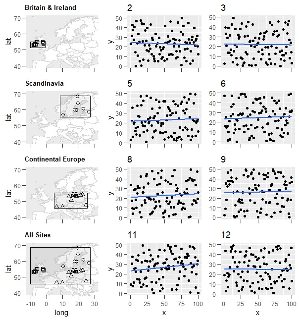
您的示例图P2、P3、P5、P6、P8、P9、P11和P12仍然无法正常工作。请考虑更新您的问题以进行更正。如果您仍然遇到问题，可以考虑使用@bVa制作的类似命名的图表进行替换。此外，您的第一次尝试使用：library(gridExtra)和grid.arrange(P1, P2, P3, P4, P5, P6, P7, P8, P9, P10, P11, P12, nrow=4)非常好，因为（在有工作图形的情况下）它很好地突出了不一致缩放的问题，即当最后一行图表具有x轴文本而其他行没有时。您可能考虑将其放回。 - krads

2个回答

1

这个来自@slizb的简洁明了的答案几乎完全满足您的需求： https://dev59.com/ImYr5IYBdhLWcg3w6eQ3#19321139 唯一的区别是@slizb在示例中展示的解决方案是单列网格布局，而您想要的是4行3列布局。

全部归功于@slizb，因为我只添加了您的数据并在最后一行中将ncol = 1更改为nrow = 4。 如果这解决了您的问题，请给@slizb点赞，而不是给这个答案点赞，因为我不能为这样微不足道的编辑声称功劳。

plots <- list(P1, P2, P3, P4, P5, P6, P7, P8, P9, P10, P11, P12)
grobs <- list()
widths <- list()

#collect the widths for each grob of each plot

for (i in 1:length(plots)){
  grobs[[i]] <- ggplotGrob(plots[[i]])
  widths[[i]] <- grobs[[i]]$widths[2:5]
}

#use do.call to get the max width

maxwidth <- do.call(grid::unit.pmax, widths)

#asign the max width to each grob

for (i in 1:length(grobs)){
  grobs[[i]]$widths[2:5] <- as.list(maxwidth)
}

# plot

#do.call("grid.arrange", c(grobs, ncol = 1))
do.call("grid.arrange", c(grobs, nrow = 4))

- krads

感谢@krads指导我找到了这个解决方案，并对我的编辑进行了修改。这对我提供的示例有效，但不适用于我实际需要完成的更复杂的示例。我已经修改了我的帖子，包括我正在处理的真实数据。您会发现grobs无法用于这些图表。 - DJ-AFC

顺便提一下，在某些标题中的“...SUM_DIFF”和“...SUM.PERCENT”字段未提供。您能否将其添加到示例中，删除或替换？否则会出现错误，无法再现。 - Jon Spring

抱歉 - 我已经将其删除。 - DJ-AFC

网页内容由stack overflow 提供, 点击上面的

可以查看英文原文，
原文链接

- bVa · Accepted Answer

另一种解决方案是使用patchwork包(thomasp85/patchwork，来自github)，您可以轻松完成。

我无法绘制P2、P3、P5、P6、P8、P9、P11和P12图形，因此我创建了模拟数据。

# mock data 
library(tidyverse)
data <- lapply(c(2,3,5,6,8,9,11,12), function(k) {
  data.frame(x = seq(1, 100, 1),
             y = runif(100, 0, 50),
             label = k) %>%
    ggplot(., aes(x, y)) +
    geom_point() +
    geom_smooth(method = "lm", se = FALSE) +
    ggtitle(k) +
    theme(axis.ticks.length = unit(0.2, "cm"))
})

p2 <- data[[1]] +
  theme(axis.title.x = element_blank(),
        axis.text.x = element_blank())

p3 <- data[[2]] +
  theme(axis.title = element_blank(),
        axis.text.x = element_blank())

p5 <- data[[3]] +
  theme(axis.title.x = element_blank(),
        axis.text.x = element_blank())

p6 <- data[[4]] +
  theme(axis.title = element_blank(),
        axis.text.x = element_blank())

p8 <- data[[5]] +
  theme(axis.title.x = element_blank(),
        axis.text.x = element_blank())

p9 <- data[[6]] +
  theme(axis.title = element_blank(),
        axis.text.x = element_blank())


p11 <- data[[7]] 

p12 <- data[[8]] +
  theme(axis.title.y = element_blank())

这是绘图的代码：

devtools::install_github("thomasp85/patchwork")
library(patchwork)
# PLOT
P1 + p2 + p3 + 
  P4 + p5 + p6 + 
  P7 + p8 + p9 + 
  P10 + p11 + p12 + 
  plot_layout(ncol = 3)